🌐 The dynamic page (htm suffix) relays real-time data from sources worldwide.
↗
🔄 To ensure you see the latest information, press CTRL+F5 to refresh the page.
📄 The static PDF version does not allow online search, playback, or sharing.
⏲️ Loading times may vary depending on your internet connection. The ↗ symbol indicates links to external references.
▤ Last updated: 2026-07-23 at 12:05 UTC ⭐ Review this page @ DXZone
Real-time propagation conditions by HF Activity Group↗
The bar above shows the global HF score (0–100) for the 17m, 15m, 12m, and 10m bands.
The global HF score graph below was designed to show dynamic variability over time due to varying levels of solar and geomagnetic activity.
Peaks indicate good global average propagation conditions, while dips indicate poor conditions. The red line represents a 48-hour global trend for reference.
What is Radio? — Radio is a type of electromagnetic (EM) energy that propagates as waves.
What is an electromagnetic (EM) wave?
An electromagnetic (EM) wave↗ is a disturbance in electric field↗ and magnetic field↗ that may propagate through space at the speed of light (~3×10⁸ m/s in a vacuum). These waves are generated by accelerating charges or high-frequency currents and carry energy across distances.
Figure 1.1: Electromagnetic Wave
Figure 1.2: A wave characterized by frequency ↗ and wavelength ↗
Frequency (f): Cycles per second (Hertz, Hz). Wavelength (λ): Distance between successive wave crests. Formula: c = f*λ, where c is light speed.
Absorption↗: The conversion of radio wave energy into heat and electromagnetic noise through interactions with matter.
Amplitude↗: The maximum extent of a vibration or oscillation, measured from the position of equilibrium.
Attenuation↗ (Path Attenuation | Path Loss): The weakening of a signal as it travels over a distance.
Diffraction↗: Waves bend around obstacles, allowing them to spread behind them.
Dispersion↗: Separation of waves at different angles of refraction ↗ of different frequencies/wavelengths.
Fading / Shadowing↗: Signal strength fluctuations (QSB).
Electromagnetic Field | Electromagnetic Radiation↗: Electric and magnetic components that oscillate perpendicular to each other.
Field Intensity↗: The strength of the wave's electric or magnetic field, typically measured in (Volt/m) or (Ampere/m).
Frequency↗: The number of cycles (peaks) per second (Hertz abrv. Hz).
Interference↗: Waves superpose to form a wave with different amplitudes, causing constructive or destructive interference.
Radio noise ↗: Unwanted random radio frequency signals that are always present in a communication system, alongside the desired radio signals.
Polarization↗: The orientation of the electric field of the wave, which can be linear, circular, or elliptical.
Power Density↗: The amount of power transmitted per unit area, typically measured in watts per square meter (W/m²).
Ray↗: The direction of wave propagation, often conceptualized as a line along which the energy of the wave travels.
Signal-to-Noise Ratio (SNR)↗: A measure comparing the level of a desired signal to the level of background noise, expressed in decibels (dB). A higher SNR indicates a clearer and more distinguishable signal from the noise.
Reflection↗: Waves bounce off a surface, where the angle of incidence equals the angle of reflection.
Refraction↗: Waves bend as they pass from one medium to another due to a change in wave speed, governed by Snell's law.
Scattering↗: Waves spread out in different directions due to interaction with particles or rough surfaces, leading to the diffusion of the incident wave.
Spectrum↗: The range of frequencies or wavelengths of electromagnetic waves, from radio waves to gamma rays.
Standing wave↗: A wave that oscillates in time but whose peak amplitude profile does not move in space.
Wave interference↗: Combine coherent waves by adding their intensities or displacements, considering their phase difference.
Wavefront↗: A surface of constant phase of the wave, which can be thought of as the leading edge of the wave moving through space.
Wavelength (λ)↗: The distance between consecutive peaks of a wave.
Propagation of electromagnetic waves Light and radio waves are examples of electromagnetic radiation that usually travels in straight lines. Long-distance communication requires waves that go beyond the horizon. Earth’s atmospheric layers and solar‑terrestrial interactions can help us understand irregular wave travel, even though it seems complex. Several factors influence radio propagation, including reflection, refraction, and diffraction. These factors depend on the medium and objects in the path of the radio waves. Signal distortion can happen when signals take different paths or mix together.
The key difference between Radio and Light is that light waves are more easily affected by obstacles and atmospheric conditions due to their shorter wavelength.
Figure 1.5 shows the electromagnetic spectrum, going from low to high frequency (long to short wavelength).↗
Figure 1.5: The electromagnetic spectrum; The radio spectrum is on the left side.
Figure 1.6 expands the portion of the radio spectrum, going from low to high frequency (long to short wavelength).↗
Figure 1.6: The chart above divides the radio spectrum into 12 bands (ELF—THF) ranging from 3 Hz to 3 THz. The microwaves are divided into sub-bands: L, S, C, X, KU, K, Ka, V, W, and G.↗
Radio Communication Circuit
Radio frequencies (RF) are transmitted as electromagnetic waves, enabling long-distance communication. A transmitter induces currents in an antenna. These signals are converted into radio waves.
The radio waves propagate away from the transmitting antenna.
Receiving antennas capture these waves and convert them into electrical signals, which are used to reproduce audio, video, or other data.
Figure 1.7: The Path of Wireless Communication
The rebirth of skywave HF radio
Skywave HF radio usage declined in the 1960s due to ever-changing ionosphere, interference, and bandwidth limits, leading to the rise of satellite technology (since 1957).↗
Between 1965 and 2020, satellite system issues—high costs, outages, and complex infrastructure—revived interest in HF radio. Advances like digital modes↗, automatic link establishment (ALE)↗, and spread-spectrum↗ have improved communication reliability via skywave, making it popular again for long-distance and emergency communications.
Advantages of Skywave over Satellites:
Remote Reach: Skywave covers areas without satellite access.
Infrastructure-Free: No infrastructure needed; ideal for emergencies.
Chapters 7—13 discuss all of these concepts. Click on the links above to learn more about each of the variables affecting HF propagation.
Chapter 2. Monitoring Ham Band Activity
Monitoring real-time ham radio activity is a reliable indicator of current band conditions. In the past, we manually scanned the radio spectrum with analog receivers. This was a time-consuming and often inefficient process. Today, advanced tools enable efficient assessment of various HF bands, both globally and regionally. By combining multiple methods and tools, you can enhance your understanding of the basics of HF band propagation conditions and ensure a more accurate assessment. The following table summarizes the proposed methods, applications, and tools.
Table 2.1: Methods, Applications, and Tools to Monitor HF Band Conditions↗
Social Media and Forums: operators share current band conditions and experiences.
2.1 Real-time ham band activity using the internet ↗
The most popular tools that show ham band activity include DX clusters, DXMAPS, DXview, DX spots, and DXFun. DX Clusters are the infrastructure, DXMAPS emphasizes specific QSOs and contests, DXView focuses on general band openings, and DXFun shows DX spots.
DX Clusters↗ are global networks that aggregate and share what stations they hear. This helps other users know which radio bands are active and where signals are coming from. By looking at this info, radio operators can assess how far their signals might travel. It’s a useful tool, but not always perfect—local variables often can still affect signals.
Figure 2.1: An illustration of DX Clusters by DALL-E AI image generator
DXMAPS provides real-time charts of reported QSOs (contacts) and SWLs (shortwave listeners) across amateur bands.
Figure 2.2: QSO/SWL real time information by Gabriel Sampol, EA6VQ
Figure 2.2 shows propagation paths that may help users analyze band conditions and contest performance effectively. Registered users can send formatted DX Spots for easier identification. Propagation mode identification is available for high bands, above 28 MHz.
The DXView map (Figure 2.3 below) shows real-time ham band activity. This visual aid helps identify open bands and communication modes ↗.
Figure 2.3: Real-time Ham Band Activity First click on the above map; then you may click on "Perspective," filling in your QTH location.
The DXView map helps identify open HF bands and communication modes based on real-time activity from the last 15 minutes on 11 ham bands (1.8–54 MHz). It compiles data from online sources such as WSPRnet, Reverse Beacon Network (RBN)↗, and DX Cluster. Data determines if a path supports SSB (SNR > 10 dB), CW (SNR > -1 dB), or only digital modes (decoding down to about -28 dB SNR). The DXView website provides a guide on interpreting the map and selecting band colors.
DX spots are real-time reports generated by multiple operators indicating the current state of HF propagation. Radio operators can communicate effectively by analyzing these spots and selecting open ham bands.
DXFun spots activity up to the recent 60 minutes. It compares amateur activity across 13 radio bands, ranging from 1.8 to 440 MHz (160 meters to 70 centimeters).You can also view a breakdown by continent and operating mode.
Figure 2.4: A demo: Real-time Ham Band Active Spots
from all continents; all modes and breakdown of modes (CW, SSB, and digital)
Click on the above chart to view real-time data courtesy DXFun, by EC4DX-Javier, EA3EXV-Gerard, EB5IPG-Luis. ↗
FT8↗ is the most popular digital mode↗ that automatically decodes weak signals and provides real-time data on HF activity.
Tools:
WSJT-X↗: A computer program used for weak-signal radio communication between amateur radio operators.
PSK Reporter↗: A global signal-reporting network that maps signal transmission and reception in near real-time.
To monitor propagation conditions:
Use software like WSJT-X to decode FT8 signals.
Upload your reports to PSK Reporter to visualize current band conditions.
Example: A PSK Reporter chart generated on April 2, 2023, by WSJT-X software, illustrating global FT8 signal reception. The following map demonstrates a near real-time data display of band activity, propagation paths, and weak signal communication conditions.
Figure 2.5: PSK Reporter Chart of Signals Received Example Receiving station
Figure 2.6: Malahite v1.3 DSP Receiver connected to K-180WLA—Receive-only Magnetic Loop antenna (MLA)
WSPR↗ (Weak Signal Propagation Reporter) is recommended to test propagation paths on the ham bands.
It is vital for ham radio because it enables operators to study long-distance signal propagation using extremely low-power transmissions. It helps test antenna performance and band conditions without requiring two-way communication. By uploading reception reports to WSPRnet, users contribute to a global network that maps real-time propagation paths.
The following are useful links:
WSPRnet,
WSPR Rocks, and
WSPR Live.
Listening to the NCDXF Beacon Network is beneficial for DX station hunting.
Eighteen worldwide beacons operate on five bands: 20, 17, 15, 12, and 10 meters.
Figure 2.7: NCDXF beacons map—All use standardized antennas and power levels.
The above is a map of the NCDXF Beacon Network, which operates on the frequencies: 14.100, 18.110, 21.150, 24.930, and 28.200 MHz. Receiving readable signals on these frequencies can indicate open bands.
Beacon IDs are callsigns in CW, followed by a carrier decreasing in four power levels: 100, 10, 1, and 0.1 Watts. If you can hear the weakest 0.1-Watt signal, it suggests good propagation or a low-noise location. The NCDXF website provides further details for operators.
Tune between 28.2 and 28.3 MHz for additional beacons operating full time.
2.4 Compare various antennas at your station to assess HF propagation conditions ↗
This activity requires hands-on experience and a basic understanding.
Using different antennas at your station helps assess HF propagation conditions by comparing received signal levels and signal-to-noise ratios (SNR). Switch between dipoles, verticals, and loop antennas to receive signals from beacons.↗
Observe variations in signal strength and clarity:
Monitor signal clarity from various distant stations on different bands using different antennas (e.g., dipole, vertical, loop).
Compare reception: Note variations in signal strength across different antennas and bands, as well as the SNR.
Analyze signal quality: Observe signal quality (e.g., fading, noise levels) for each antenna.
If you consistently receive stronger signals on 20 meters with a vertical antenna compared to weaker signals with a dipole, it may indicate favorable vertical wave propagation conditions. Conversely, if 40 meters performs better with the dipole, that could suggest more favorable horizontal wave propagation on that band.
By systematically observing these factors, you can gain valuable insights into current HF propagation conditions and optimize your antenna choices for specific bands and destinations.
2.5 Monitor bands using public remote SDR receivers
WebSDR, KiwiSDR and OpenWebRX offer online access to remote receivers.↗ These platforms allow users to monitor global HF signals without local equipment. Both support multiple users and offer real-time spectrum and waterfall visualization. However, their user interfaces and functionalities differ, with each platform having unique advantages to suit various needs and preferences. The following example demonstrates the Wideband WebSDR at the University of Twente, Enschede, NL↗. The visual spectrum and waterfall display enable users to monitor and analyze signals from remote locations.
Figure 2.8: Real-time waterfall display for a wide radio spectrum, frequency range of 0-29 MHz, with the ability to resize the width down to 250 KHz.
Alternatively, choose a remote receiver from the following maps:
Figure 2.9: WebSDR Global Map showing locations worldwide
Users can select a receiver to remotely monitor HF signals, access live waterfall displays, and tune into specific bands.
Figure 2.10: Global map of Kiwi SDR receivers showing locations worldwide
Users can select stations to explore propagation conditions and compare band activity at different geographic locations.
High Frequency (HF) radio enables long-range communication by skywave propagation. However, its reliability shifts constantly due to various key factors. For radio operators, forecasters, and emergency responders, this unpredictability is both a challenge and a chance to use forecasting tools to improve planning and performance. ↗
Forecasting Requires Scientific Insight
Two complex natural systems influence HF propagation:
The Sun emits variable amounts of photon radiation and charged particles.
The ionosphere refracts HF waves. Its structure determines which bands open, at what times, and for how long.
Forecasting is not guesswork; it’s a scientific estimation based on known processes.
Evolution of forecasting techniques
Remarkable advancements in space technology↗, software-defined radio (SDR)↗, and the internet have revolutionized our understanding of radio wave propagation. Before the 1990s, propagation charts and reports were often published in amateur radio magazines. Today, real-time solar indices and computer programs provide accurate, up-to-the-minute propagation data via online tools↗.
How to determine HF band conditions? (short primer)
The MUF, based on ionograms, plays a key role in determining HF propagation conditions. Viewing the activity map on the airwaves matches and complements the information necessary to understand current communication conditions.
Real-time tools such as WebSDR, PSK Reporter, the activity map, and the MUF map provide a snapshot of current conditions, whereas forecasting tools attempt to predict what will happen next. ↗
All these tools are useful for planning contests, long-distance communication (DXing), field operations, emergency preparation, and selecting the optimal band for a specific time of day.
The terms "forecasting" and "prediction" differ primarily in their time frames and methodologies.
Forecasting: Short-term estimations based on current data (e.g., "Conditions will improve in the next hour").
Prediction: Long-term estimates based on trends (e.g., "Better 40-meter conditions expected next month").
Practical Forecasting and Prediction of HF Propagation
Line of Sight exists when radio signals pass directly between two stations with no obstacles in between. This mode works well for short-range transmission at higher frequencies, often within a few kilometers of the visual horizon. Signals cannot follow the curvature of the globe.
Non-LOS propagation↗ occurs if obstacles exist; radio waves may reflect off conductive surfaces like buildings or mountains.
2. Ground wave↗ or surface wave propagation: Effective below 2 MHz; influenced by terrain and conductivity.
AM radio stations use ground wave propagation during the day.
Vertically polarized surface waves travel parallel to the Earth's surface and can cross the horizon.
Geologic features and RF absorption by the earth attenuate ground wave transmission.
Ground waves fade faster as their frequency increases. Range is determined by the type of surface (ground, soil, salinity, rough or smooth sea) and the maximum attenuation that allows for reliable radio communication.
See practical approximate formulas.
Ground wave is effective below 1 MHz over salty smooth seawater or conductive ground but is ineffective above 2 MHz.
The Skip Distance illustrated in Figure 4.1 refers to a region with no reception between ground wave and skywave coverage. It is calculated using the following formula:
where Dskip is the Skip Distance, h is the height, fMUF is maximum usable frequency, and fc denotes the critical frequency↗.
Special cases:
Gray line (greyline): Utilizes the twilight zone around Earth separating daylight from darkness.
NVIS: Near Vertical Incidence Skywave operates at 2–8 MHz, using low horizontal antennas to address skip / dead zone.
Sporadic E: In late spring or early fall, low VHF (30 to 150 MHz) signals can be unpredictably refracted back to Earth.
Aurora: Enhanced solar wind could create aurora near polar regions. The aurora reflects radio waves from much over 30 MHz to the full UHF band (300–3000 MHz). These signals show strong fading (QSB), which is a type of bubbling sound. As a result, only narrow-band modes like CW and digital are reliable for DX communications.
Please note: Currently, this project excludes rare radio wave propagation modes, such as:
Tropospheric scatter
Meteor scatter
Backscatter
Moon Bounce (Earth–Moon–Earth or EME)
Table 4.1: Summary of HF basic propagation modes
Mode
Distance Range
Key Features
Frequency Range
Line-of-Sight
Short (a few km)
Direct signal path with no obstructions
Above 30 MHz
Ground Wave
Up to 100 km
Follows Earth's surface; best over seawater
Below 2 MHz
Skywave
Global (1000+ km)
Refracted by the ionosphere; supports long-distance
Among these modes, skywave propagation is the most versatile for HF bands. The upcoming chapters detail the factors affecting skywaves.
Chapter 5. How does the Sun affect radio communications?
The Sun affects how radio waves travel. Figure 5.1 illustrates how the solar EUV radiation ionizes the upper atmosphere, creating the ionosphere—a dynamic region that enables HF skywave communication.
Figure 5.1: An illustration of ionosphere generation and its effect on radio waves
Video clip: The dance of radio waves within a vibrant airglow. Solar storms intensify the ionosphere's beauty, while Earth's weather below adds to the unique destination.
HF radio waves transmitted from Earth to the ionosphere cause the free electrons to oscillate and re-radiate, resulting in wave refractions↗.
The ionospheric refractive index is similar to that in geometrical optics ↗. Figure 6.3 illustrates light refraction in a glass prism.
Figure 6.3: Light refraction in a glass prism
A prism bends blue light more than red, creating a rainbow. Glass prisms have a higher refractive index for blue light than red (typically 1.5–1.8).
In contrast, ionospheric plasma has a refractive index slightly less than one and bends low HF bands (3–10 MHz) more than high HF bands, as shown in Figure 6.4.
Figure 6.4: Ionospheric refraction of radio waves.
Conclusion: The ionosphere refracts lower frequencies more.
The refractive index plays a key role in radio wave propagation, influencing how signals bend in the ionosphere. Changes in electron density—often caused by solar activity—can disrupt these signals, making it essential to monitor these conditions for stable communication. Refer to section 7.4.
Regional Propagation Factors
Chapter 7: Ionospheric Influence
The ionosphere, composed of ions and electrons, plays a vital role in radio communication by refracting skywave signals.
Figure 7.1: Ionospheric regions during daytime fade at night. Sub-chapter 8.3 explains this 24-hours cycle.
"Ionospheric regional conditions" refer to the variations in the ionosphere's electron density and behavior, which can affect radio wave propagation and navigation systems. These conditions can be influenced by factors such as solar activity, geomagnetic storms, and local atmospheric phenomena, leading to disturbances that impact communication and navigation technologies.
It’s common to present the order of ionosphere regions affecting HF skywaves from the highest region downwards, as follows:
The F region, located between 150 and 800 km above the Earth, enables long-distance HF communication in the 3.5 to 30 MHz bands.
This region consists of ionized↗
atomic oxygen (O+) hydrogen (H+) and helium (He++) with the highest free-electron density up to 1012 electrons/m³ excited by the solar EUV↗. It splits during the day into two sub-regions, F1 and F2, which merge and fade away after sunset.
The E region, located between 90 and 150 km above the Earth, dissipates a couple of hours after sunset.
This region consists of ions such as O2+, O+ up to 1011 electrons/m³ excited by the solar EUV.
During intense Sporadic E(Es)↗ events (particularly near the equator) it sporadically refracts frequencies in the 50-144 MHz bands.
The D region, located 50–90 km above ground, is active during the daytime and disappears at sunset.
In this region, solar UVC↗ at 121.6 nm excites nitric oxide ions (NO+),
up to 1010 electrons/m³. This causes low HF (~3–10 MHz) to be absorbed during daylight hours, preventing frequencies lower than the lowest usable frequency (LUF) from reaching higher E and F regions (Figure 7.9).
Additionally, two D region phenomena may disturb "normal" propagation conditions
Intense bursts of X-rays from intense solar flares↗ dramatically increase D region ionization, raising its electron density. This causes radio signals to be absorbed at increasingly higher frequencies—a phenomenon known as a radio fadeout/blackout, which can persist from several minutes to a few hours.
Why does the density of free electrons increase sharply with height between 50 km and 250 km?
The density of free electrons results from a balance between ionization ↗ (due to solar EUV) and recombination ↗ (ion-electron recombination events). The F region gets most of the UV radiation compared to the lower E and D regions, while the rate of electron-ion recombination is much faster in the lowest D region (due to the higher gas density). As a result, the free-electron density of the high-set F region (at noon) is significantly higher than that of the E and D regions. At most, only one thousandth (1/1000) of the neutral atmosphere is ionized.
7.2 Long and Mid-Range Skywaves
Figure 7.3 shows skywave refractions from the F and E ionospheric regions.
Figure 7.3: Multi refractions of radio waves in the ionosphere.
The F region refracts HF (3-30 MHz); Figure 6.4 illustrates the difference between low and high HF bands refraction. The E region sporadically refracts low VHF (50-150 MHz).
Long-range skywave propagation typically employs low transmission angles that correspond to high incident angles.
Figure 7.4: Transmission angle (α) and incident angle (θ)
A low transmission angle, which means the transmitted beam is nearly horizontal, enables refractions at higher frequencies and over longer distances. However, using real antennas at frequencies below 30 MHz to achieve low-angle radiation of less than 5 degrees can be extremely challenging.
7.3 Multi-hop Propagation
The ionosphere↗ refracts skywaves↗ in complex multiple modes
Figure 7.5: Complex skywave modes:
F Skip / 1F1E, E-F Ducted, F Chordal, E-F occasionalspread F↗ and sporadic E↗.
This figure extends Fig.2.4 of ASWFC ↗.
The diagram illustrates various modes of radio wave propagation in the ionosphere, such as ionospheric tilt, chordal mode, ducted mode, sporadic E, F skip, 1F1E, and 1F1Es1F. It emphasizes how radio waves interact with the E and F regions, depicting their travel paths across long distances.
Four characteristic frequencies, foF2, MUF, OWF, and LUF serve as indices for skywave propagation conditions ↗.
7.4.1 The F2 region critical frequency↗ (foF2) is the highest frequency below which a radio wave is reflected/refracted by the F2 region at vertical incidence, independent of transmitting power. Why is there a limit? If the transmitted frequency exceeds the plasma frequency of a region, then the free electrons (in that region) cannot respond fast enough—they are unable to re-radiate the signal. Higher frequencies escape into space.
Figure 7.6: Vertical refraction from region F2 depends on the critical frequency f0 of that region
Day vs. Night and Geographical Locations: The critical frequency varies with latitude and the day due to increased ionization from solar radiation ↗. At night, the MUF decreases.
The graph below shows how the critical frequency varies with latitude during the day and night.
Day Hemisphere: The red curve (F2 region) peaks around 18 degrees latitude, forming an "equatorial anomaly." ↗ The blue curve (E region) remains relatively flat.
Night Hemisphere: The red curve shows a "mid-latitude trough" around 60 degrees latitude. Gradually growing towards the equator. The E region dissipates at night.
Seasonal Variations: The critical frquency is higher in summer due to the Sun being directly overhead and lower in winter.
Solar Activity: High solar activity can increase the MUF by enhancing ionospheric ionization.
Geophysical conditions: Factors such as geomagnetic activity and atmospheric tides can also have an impact.
Between the years 2005 and 2007, the global average critical frequency (foF2) ranged from 1.8 MHz to 11 MHz, with an overall average of 7.5 MHz.
7.4.2 The Maximum Usable Frequency (MUF) ↗ (synonym: Highest Possible Frequency—HPF) is an index for forecasting propagation conditions. It is the highest frequency you can use to send radio signals successfully. The MUF depends on the angle at which those signals are transmitted but is independent of the transmitting power.
Figure 7.9: Radio wave absorption occurs during the day at frequencies below 10 MHz.
LUF, also known as the absorption-limited frequency (ALF), is a soft frequency limit, unlike the sharp cut-off of the MUF.
The D region absorbs frequencies below the LUF during the day. At night, the D region does not exist, so there is no low-frequency limit.
NVIS provides the solution for the dead zone (between ground wave and skip). It is the only solution for communication coverage in hilly and/or jungle areas over short distances of a few hundred kilometers.
Figure 7.10: How NVIS provides communications within a hilly area.
Typical operating frequencies are 2-4 MHz at night and 4-8 MHz during day.
NVIS requires suitable antennas (like a low dipole at hight of 0.1-0.25 wavelengths) to improve vertical radiation and reduce lower-angle radiation, contrary to what is customary for long-range communication.
NVIS offers enhanced resistance to fading (constant signal level), and minimal attenuation, making it suitable for low transmit power levels and omnidirectional coverage, allowing flexibility in setup and placement.
To avoid skip zones on 40 m band use NVIS when foF2 is higher than 8.5 MHz. Switch to 80 m if the day is on the downward slope. Optimize antenna radiation pattern for the desired takeoff angle. Optimum NVIS height for horizontal dipoles: 0.18–0.22λ for TX and 0.16λ for RX ↗.
The "gray line" (Americam English, grey British) is the twilight zone around the Earth separating daylight from darkness. Propagation along this zone is highly efficient because the D region, which absorbs HF signals during the day, vanishes quickly on the sunset side and hasn't formed yet on the sunrise side. Ham radio operators and shortwave listeners can optimize long-distance communications by tracking this twilight zone.
Figure 7.11: Ionospheric Regions and Gray Line
The height of the F and D regions↗ shown above is exaggerated in comparison to Earth dimensions.
Figure 7.12: A recent gray/grey line chart with Sun and Moon positions courtesy of Timeanddate ↗
Some radio operators use specialized gray line map ↗ to predict when the gray line will pass over their location, as well as the best frequencies and modes of propagation to apply at that time. Overall, gray line propagation is a fascinating and useful phenomenon that has the potential to open up exciting opportunities for long-distance radio communication.
7.7 Ionospheric regional conditions—summary
This chapter examines ionospheric regions, distributions of free electrons, critical frequencies, and specific propagation modes, NVIS and grayline.
Table 7.1: A summary of ionospheric regional conditions at noon
The following is supplemental material that may help you understand ionospheric dynamics. Figures 7.13 and 7.14 show ionospheric physical conditions, temperature distribution, free electron density, pressure, density, gas compositions, ionic compositions, chemical reactions, and transport phenomena (horizontal and vertical winds).
Figure 7.13 shows:
Temperatures distribution due to low or high solar flux
Free electron density
Ionic compositions.
Not shown on the figure:
Gas pressure and density
Gas compositions
Chemical reactions
Winds: horizontal and vertical
Figure 7.13: Ionospheric physical conditions
Figure 7.14 below shows the distribution of major ionic compositions.
Figure 7.14: Ionospheric composition during daytime solar minimum adapted from Johnson, 1966, Figure 1.
In his 1966 study on the ionosphere, C.Y. Johnson ↗ primarily focused on the ionic composition of the dayside ionosphere during solar minimum. He found that O+ (oxygen ions) are the most dominant ions, especially at altitudes below 250 kilometers, with H+ (hydrogen ions) becoming more prevalent at higher altitudes. He also observed the presence of He+ (helium ions) at even higher altitudes, although in much smaller concentrations than O+ and H+.
Chapter 8. Regional HF Propagation Conditions
Regional propagation conditions (in a specific geographic area) offer information about individual operators' experiences based on observed foF2, MUF, and LUF values between two locations. The next subsections explain how these values are measured and presented.
The ionosonde, also known as the chirpsounder ↗ (developed in 1925), is an HF radar that sends short pulses of radio waves into the ionosphere to find the most optimal frequencies for HF communication. It calculates the time it takes for pulses to return and then plots the height (derived from the time delay) versus frequencies to produce an ionogram. An ionosonde sweeps the HF spectrum from 2 to 30 MHz, raising the transmitted frequency (Tx) by about 100 kHz per second and digitally modulating it in 25 kHz increments. Matching receivers (Rx) detect and analyze echo signals, as seen in the next figure.
Figure 8.1: Basic ionosonde types are vertical and oblique sounding
Every 15 minutes, ionosonde stations around the world report real-time data via the internet.
Figure 8.2: Global map of Giro digisondes as of 2017↗
Some stations aren't always active. Since 2021, real-time ionosonde data sharing has reduced in countries such as Russia, China, Japan, and others. Thus, significant regions of the globe are not yet covered with ionosonde stations, as shown on the above map.
An ionogram is a visual representation of the height of the ionospheric refraction of a specific HF radio frequency. It shows the plasma density distribution in ionospheric regions at various altitudes (48–800 km).
Ionograms typically display two key elements:
Horizontal Lines: These lines indicate the virtual height at which an ionosonde pulse is echoed, varying with the operating frequency.
The ionogram above illustrates the ionospheric E and F2 regions. The red curve shows ordinary refraction, and the green curve shows extraordinary refraction, due to the ionosphere's anisotropic nature causing double refractions (birefringence)↗.
While this provides a simplified explanation, the reality is that the ionosphere is neither uniform nor stable, perpetually changing over time. Consequently, researchers developed the Digisonde Directogram to identify ionospheric plasma irregularities.
8.3 Day-night: Regular diurnal (daily) cycle
Earth’s daily cycle repeats every 24 hours, driven by the Sun’s influence on atmospheric ionization.
The figure 8.5 below illustrates typical diurnal patterns of heights above the ground and duration after sunset.
Figure 8.5: Diurnal cycle of ionospheric regions
The F region exhibits the highest electron density, which decreases at night. The E region, with a lower density during the day, begins to decline a few hours after sunset. The D region disappears entirely at sunset.
All the characteristic frequencies increase at dawn and decrease at dusk, with LUF dropping to zero at sunset (Figure 8.6).
Figure 8.6: Typical diurnal cycle based on Naval Postgraduate School training materials↗
FMUF: F region maximum usable frequency OWF: optimum working frequency EMUF: E region maximum usable frequency LUF:
The lowest usable frequency is due to D-region absorption, which limits the window of useful frequencies ↕
Dynamic variability: Anomalies and disturbances
Figure 8.7: Observed vs. predicted foF2 Based on Australian Space Weather Alert System (ibid. Fig 3.3) ↗
Figure 8.7 compares the observed foF2 (solid black) and predicted foF2 (dotted red) over four days. On the second day, around noon, there is a significant increase in observed MUF, surpassing the predicted trend. This could indicate increased ionosphere activity or favorable propagation conditions. HF propagation conditions decreased as observed frequencies fell below predicted levels over the next few days. The contrast between the initial enhancement and subsequent suppression highlights the dynamic variability of ionospheric behavior over time.
Figure 8.8: Ionospheric region heights vary seasonally and diurnally.
Figure 8.8 illustrates the increase in the height of the F region in the summer. This may result in chages of the MUF and the ability of that region to refract radio waves due to falling free electron density. Additionally, the D region's height remains stable while absorbing more ionizing radiation ↗, leading to increased absorption and a higher LUF. As a result, HF band conditions above 10 MHz are better in the summer and near the equator, while bands below 10 MHz are better in the winter and at mid-latitudes (Table 8.1).
Table 8.1: Summer versus winter (daytime)
Geographic latitude: degrees
Summer F2 region height
Summer MUF
Summer D region height
Summer LUF
Mid-latitude: 30-60°
Higher
Lower
Same
Higher
Equatorial: 0-20°
Higher
Higher
Same
Higher
Summer anomalies↗ can cause plasma irregularities in the ionosphere's mid-latitude F region in both hemispheres. Seasonal changes significantly impact ionization, with summer frequently bringing instabilities known as mid-latitude spread-F due to increased solar radiation. The Arecibo Radio Observatory in Puerto Rico observed anomalous electron density irregularities during such an event, extending above the ionosphere's stable topside (Figure 8.9). ↗
Figure 8.9: Electron density anomaly at mid-latitudes↗
The top figure shows both the E and F regions on the same scale and the bottom figure shows E region in an expanded scale
MUF Seasonal and Solar Activity Influences
Anomalous seasonal variation: Mid-latitudes can experience the "seasonal anomaly," where winter MUFs are higher than summer MUFs, especially at solar maximum.
Geographical influence: Equatorial MUF is primarily influenced by the "fountain effect" and vertical plasma drifts, which are stronger in the summer.
Solar activity impact: While seasonal variations are complex, solar activity can significantly alter MUF, with the seasonal anomaly at mid-latitudes becoming more pronounced at higher solar activity levels.
MUF 3000 km map: HF propagation conditions at a glance updated every 15 minutes; Provided by KC2G There is also an animated version showing the last 24 hours.
Online MUF 3000 km propagation map ↗updated every 15 minutes
This near-real-time online map may assist radio amateurs in finding the best frequencies for contacts by displaying HF propagation conditionsat a glance.
The map shows the calculated MUF based on ionograms.
A radio path of 3,000 km is being considered for unification.
The colored regions of this map, defined by iso-frequency contours, illustrate the MUF expected to refract off the ionosphere along a 3000 km path. The map also includes the position of gray line.
The ham bands are designated by iso-frequency contours: 5.3, 7, 10.1, 14, 18, 21, 24.8, and 28 Mhz.
For example, if a given area on the map is greenish and lies between the contours labeled "10" and "14," the MUF in that location is around 12 MHz.
The raw data is MUF calculated from data collected by ionosondes, which are represented by numbered colored discs that show their location. A number inside a disc indicates the calculated 3000km MUF from the critical ionospheric frequencyfoF2. The information from selected stations is compiled by Mirrion 2↗ and GIRO↗, and processed by the International Reference Ionosphere (IRI) model ↗ (produced by a joint task group of COSPAR↗ and URSI↗.
The MUF along a path between any two locations shows the possibility of long-hop DX between those points on a given band. For example, if the MUF is 12MHz, then 30 meters band and longer will work, but 20 meters band and shorter won't. For long multi-hop paths, the worst MUF anywhere on the path is what matters. For single-hop paths shorter than 3000 km, the usable frequency will be less than the indicated MUF. As one gets closer to vertical, i.e., NVIS, the usable frequency drops to the Critical ionospheric frequency, (foF2, as shown in the next map).
Notes:
The accuracy of the data is insufficient for commercial radio services due to several factors:
Uncertainty in predicting ionospheric state:
Vertical sounding data introduces uncertainty when predicting the ionosphere's state.
The limited coverage of monitoring radio stations results in reliance on data processing.
Challenges of data interpolation and extrapolation ↗:
The algorithm attempts to determine the MUF (or foF2) at scattered points globally.
Accuracy is compromised when extrapolating from sparse data points.
Predictions are more reliable near measurement stations but deteriorate for distant regions.
Issues with measurement stations:
Inconsistent or conflicting data from stations may lead to unusual results when aligning measurements.
Unexpected global model changes may occur due to stations going offline or reappearing, compounded by the limited initial data points.
Restricted sharing of real-time data:
Since 2021, real-time ionosonde data sharing has reduced in countries such as Russia, China, Japan, and others.
Some ionosondes are accessible solely via NOAA, and GIRO outages could cause map updates to cease.
Events such as geomagnetic storms, elevated X-ray flares, and solar wind significantly affect the accuracy of MUF estimations derived from vertical sounding data.
While these disturbances are implicitly reflected in ionogram results, predicting band conditions remains challenging.
The propagation model is overly simplistic. It does not capture all the variables, such as blackouts due to D-region absorption and noise induced by geomagnetic storms.
Future Development: Efforts are underway to develop geospace dynamic models to mitigate these challenges.
The "MUF(3000km)" project is the result of research and development by Andrew D Rodland - KC2G, which is based on an earlier work by Matt Smith, AF7TI. WWROF financing and data from ionosonde operators all over the world, provided by GIRO ↗ and NOAA ↗ made it feasible.
Figure 8.12: Animated MUF 3000 km propagation map in the last 24 hours courtesy of Roland Gafner, HB9VQQ
NVIS online live map for vertical refraction (critical frequency foF2)
provided by Andrew D Rodland, KC2Gupdated every 15 minutes
Figure 8.13: Online NVIS Map, by Andrew, KC2G
The map's colored regions, outlined by iso-frequency contours, show the global distribution of the critical frequency for near-vertical ionosphere refraction.
Colored discs mark ionosonde stations, with numbers representing critical frequency (foF2)—the site's raw data source.
A commercial NVIS real-time map provided by the Australian Space Weather Service ↗ is updated every 15 minutes. It displays contours of the critical ionospheric frequency—foF2. There are a few differences between this map and the KC2G map, mainly due to the choice of frequencies for the contours. The KC2G map highlights ham bands. The following map, however, is designed for commercial use.
Figure 8.14: Online NVIS map courtesy of ASWFC Click on this online map to view the source page. There is further information.
Online T Index Map shows the variation of regional propagation conditions relative to the global average.↗
Figure 8.15: The T Index Map courtesy of ASWFC; Updates every 15 minutes.↗
Figure 8.15 shows a near-real-time T index difference map with four-level contours. The depressed regions (yellow and red) may lack sufficient high-frequency communication support. Click on the map to access the source. There are options for reviewing the past seven days, as well as an animated map.
The T index (transmission index "equivalent sunspot number") is used in HF propagation to assess the conditions for radio wave travel. It helps radio operators to estimate the probability of making long-distance contacts by reflecting the current state of the ionosphere. This index was created by the Australian Ionospheric Prediction Service↗. The values range from -50 to 200. Higher values correspond to ideal conditions, while lower values indicate reduced HF frequency usability.
The T index derives from foF2 measurements, which take into account ionospheric condition anomalies ↗. It compares recent measurements of regional conditions to the previous month's average global conditions to predict HF regional communication and serve as an analog for sunspot numbers.
The recent foF2 measurements at various locations of Australia, New Zealand and East Antarctica
Figure 8.16: foF2 Plots courtesy of Australian Space Weather Forecasting Centre Click on this figure to view the source page with legends.
This chart relies on events and updates whenever a flare of magnitude M1 or greater occurs. The top line indicates the recent flare time.
The chart illustrates the LUF affected by the recent significant solar X-ray flare. As shown by the color bar, the most significant impacts occur within the inner circle. The map reflects the LUF for standard 1500 km HF circuits, where communication below the LUF is uncommon, while communication above it is generally possible. Shorter circuits may exhibit higher LUF values, enabling the use of lower frequencies. Conversely, longer circuits might still experience signal fading, even at elevated frequencies.
What is TEC? TEC is the total number of free electrons present along a path between satellite and receiver.
Why is TEC important for HF propagation conditions?
TEC correlates with the critical frequency, foF2, and is therefore implemented in a variety of ionosphere models ↗. Moreover, the total electron content can provide additional information about the structure and dynamics of the ionosphere. It can detect and monitor ionospheric disturbances, such as those caused by solar flares or geomagnetic storms.
Units: 1 TEC Unit (TECU) is the number of free electrons per square meter (x1016) for a shell height of 400 km directly above a certain point. Values in Earth’s atmosphere can range from a few to several hundred TEC units.
How is TEC measured? Data is gathered from GPS receivers worldwide, observing carrier phase delays in radio signals from satellites above the ionosphere, often using GPS satellites.
Extreme Ultra Violet (EUV) radiation↗creates the ionosphere, especially the F2 region. Since EUV is fully absorbed by the ionosphere, it doesn't reach the ground, making direct measurement impossible for ground-based devices. Before the space age, scientists relied on two indirect markers to gauge the ionization levels of the F2-region. These are the solar indices:
The solar flux index (SFI) quantifies the intensity of solar radiation at 2.8 GHz (10.7 cm wavelength). ↗
Higher flux indicates greater ionization levels in the E and F regions, improving HF radio propagation conditions.
The Sunspot number (SSN) is a count of the number of dark spots seen on the Sun. ↗
Higher SSN values correlate with improved conditions on the 14 MHz band and above.
The 304 Å Index measures the solar radiation strength at 304 Ångstrom (30.4 nm) EUV, emitted primarily by ionized helium in the Sun's photosphere. This parameter has two measurements: one from the EVE instrument↗ on the Solar Dynamics Observatory (SDO) and the other from the SEM instrument on the SOHO satellite. It accounts for about half of the ionization of the F region in the ionosphere and loosely correlates to the SFI. The background SFI level is typically around 134 at solar minimums and can exceed 200 or more at solar maximums. It is updated hourly.
Solar X-ray flares (1–8 Ångstrom / 0.1—0.8 nm) are measured by instruments onboard GOES satellites.
Intense X-ray flares can cause enhanced ionization at the D region, leading to communication disruptions and blackouts.
Understanding the Correlation between Sunspots and Solar Flux:
Sunspot number records have been traced back to the 17th century but are often subject to interpretation. The solar flux at 10.7 cm wavelength (2,800 MHz) aligns closely with daily sunspot numbers, making both databases interchangeable.
The 10.7 cm Solar Flux data is more stable and reliable compared to the Sunspot Number (SSN).↗
Radio telescopes in Ottawa (from February 14, 1947, to May 31, 1991) and Penticton, British Columbia (since June 1, 1991), report solar flux density at 2,800 MHz daily at local noon (1700 GMT in Ottawa and 2000 GMT in Penticton). Corrections are made for factors like antenna gain, air absorption, solar bursts in progress, and background sky temperature.
Due to variations in solar radiation globally, even with corrections, consistent results are challenging. Thus, readings from the Penticton Radio Observatory in British Columbia, Canada, are used as a benchmark. These numbers are crucial for predicting ionospheric radio propagation.
The 10.7 cm radio flux consists of contributions from the undisrupted solar surface, active regions, and transient enhancements above the daily level. Levels are determined and corrected within a few percent.
Geomagnetic indices measure disturbances in the Earth's magnetic field, which can disrupt HF propagation by increasing atmospheric noise and weakening radio signals. These indices are crucial for understanding the potential impacts on all communication systems, satellite operations, and even power grids.
K and A are local indices
K-index↗: This index represents short-term (3-hour) geomagnetic activity at a specific geomagnetic station. It quantifies disturbances in Earth’s horizontal magnetic field by comparing geomagnetic fluctuations, measured with a magnetometer↗, to a quiet day. The K-scale is logarithmic, allowing for a more manageable representation of the wide range of geomagnetic activity magnitudes.
A-index: This index averages K values over a 24-hour period to provide a linearized view of geomagnetic activity. It is important for predicting and understanding the effects of geomagnetic storms on HF communications.
Kp and Ap are global—planetary indices.
K and A indices measure local geomagnetic activity at a single observatory.
Thirteen geomagnetic observatories at mid-latitudes are used to get a world average of the K and A indices, which are shown as Kp and Ap.
Kp: Average of K-indices from 13 observatories, indicating planetary geomagnetic activity.
Ap: Daily planetary geomagnetic activity, derived from the Kp index.
The HPo indices are less commonly referenced. The half-hourly Hp30 and hourly Hp60, developed at GFZ (German Research Center for Geosciences), offer improved time resolutions compared to the three-hourly Kp. Together with the linear versions Ap30 and Ap60, they are collectively known as the HPo index, providing near-real-time data. This higher time resolution is critical for predicting and mitigating the impacts of geomagnetic storms on various technologies. ↗
HF propagation indicators are essential tools for amateur radio operators to evaluate and predict skywave conditions.
Global indices include ionospheric noise levels, solar indices (SSN, SFI), X-ray flare activity, solar wind parameters, and geomagnetic indices. The most important indices are the Maximum Usable Frequency (MUF) and Lowest Usable Frequency (LUF), which vary by location. These indicators are all interconnected. Understanding how they are related helps operators anticipate HF propagation changes as atmospheric and solar conditions evolve.
Conclusion: High values of the solar indices SSN and SFI correlate with higher MUF. Watch a graph of the recent 30-day sunspot numbers. The current SFI: Loading solar flux data... (solar flux units; 1sfu=10-22 Watts per meter² per Hz). The HF band conditions may drop when there is significant geomagnetic activity.
Table 10.2: The geomagnetic activity indices K and A, and bad HF band conditions.
Note: The solar wind significantly influences fluctuations in the geomagnetic indices. By examining solar wind data—such as density and velocity—we can understand both the "why" and "how fast" behind these changes, allowing us to predict variations ahead of the next 3-hour K update. If you're simply determining whether the HF band is usable tonight, the local K index may suffice. However, for optimizing a specific path or timing, incorporating solar wind data becomes essential.
Table 10.3: An approximate correlation between solar flare classes, radio blackout scale, and the HF band conditions.
Solar irradiance↗ quantifies sunlight power on a surface in watts per square meter (W/m²). On Earth, it fluctuates with location, time, and atmospheric conditions. Since 1978, space-based studies show the "solar constant" varies, influenced by cycles like the 11-year sunspot cycle. Quiet and active solar events affect space weather and HF skywave propagation.
The Sun emits electromagnetic radiation↗ across a wide spectrum↗ from Gama-rays to ELF.
Figure 11.1: The solar electromagnetic spectrum, arranged left to right by wavelength from shortest to longest.
The extreme ultra violet EUV↗ generates the ionosphere. Figure 11.2 presents a typical spectrum of the solar EUV.
Figure 11.2: Spectral chart of the quiet EUV solar spectrum
This EUV spectrum was obtained by the SDO/EVE instrument during a rocket flight on April 14, 2008, at solar minimum between cycles 23 and 24. The He II peak at 30.4 nm significantly contributes to half of the ionization↗ in the Ionospheric F region.
Ref↗: ibid. Solar UV and X-ray spectral diagnostics, Fig. 11 on page 25 of 278.
11.2 Active Sun
An active sun means it is sending out bursts of energy like flares and charged particles that can mess with radio signals.↗ Solar activity is driven by the eleven-year periodic reversal of the Sun's magnetic field. It is caused by a helical dynamo in the sun's core and a chaotic dynamo near the surface that generate the sun's magnetic field. ↗
The main solar phenomena associated with HF radio propagation on Earth are:
Sunspots: last from a few days to a few months; the number of spots varies in 11-year solar cycle↗ (a deterministic chaos↗);
Solar flux at 10.7 cm (2800 MHz) ↗: a measurable indicator of solar activity that correlates with sunspots;
Solar activity observations include region-specific diagnoses. These regions are areas on the Sun's surface with strong magnetic fields, which are frequently associated with sunspots. Solar flares are most commonly seen in these regions, where magnetic energy accumulates and is suddenly released, resulting in explosive events.
Higher sunspot numbers indicate elevated solar flux levels, enhancing ionization in Earth's upper atmosphere and improving high-frequency (HF) radio wave propagation. Conclusion:more sunspots → higher solar flux → better HF communication.
Sunspots vary in shape, size, and duration, lasting from a few hours to several months.
The average number of sunspots fluctuates throughout the solar cycle, an approximate 11-year cycle of solar activity.
Left: Sunspots in visible light Right: Extreme Ultra Violet↗ (EUV 30.4 nm) Figure 11.3: Two images of the Sun (February 3, 2002) by Solar and Heliospheric Observatory (SOHO) satellite↗ courtesy of European Space Agency and NASA.
What is the reason for analyzing sunspots in both visible and ultraviolet light?
Observing sunspots in visible light allows us to see them directly with our eyes or telescopes. Using ultraviolet (UV) light reveals magnetic disturbances that are invisible in regular light. Studying sunspots in both visible and UV light helps us understand their features and the activities occurring on the Sun.
11.4 Solar storms (X-ray flares and particle events)↗
The Impact of Solar Storms on HF Communication
Solar storms can significantly disrupt high-frequency (HF) communication through radio fadeouts and blackouts, caused by solar flares and solar energetic particles (SEP).
SEP events: Mainly cause Polar Cap Absorption (PCA)↗, leading to attenuation levels that can obstruct most transpolar HF radio transmissions. In severe cases, can result in tens of decibels of attenuation.
a PCA may commence as soon as a few minutes after the flare onset and persist up to ten days.
For centuries, people have been observing sunspots without knowing what they are.
We now understand that these are symptoms of solar storms.
Figure 11.4: Solar storms consist of solar flares↗ associated with CMEs↗ Image (EUV 30.4 nm) credit: NASA, Aug. 2012; captions added by 4x4xm.
Coronal Mass Ejections (CMEs) often appear as twisted ropes. Figure 11.7 presents the model connecting solar flares with CMEs.
(B) Solar Energetic Particle Events↗ (CME ↗, SEP↗, and SPE):
A Coronal Mass Ejection (CME) is a massive eruption of charged particles and magnetic fields from the Sun's corona into the heliosphere. ↗ These powerful events, which occur more frequently near the solar maximum, can travel at incredible speeds, reaching Earth in hours or days, disrupting space weather, causing geomagnetic storms and auroras, and potentially affecting satellites, power grids, and high-frequency skywave communication. The magnetic fields of CMEs merge with the interplanetary magnetic field.
Figure 11.6: LASCO C2 image↗, taken January 2002 shows coronal mass ejection (CME) captured by SOlar and Heliospheric Observatory (SOHO)↗. Credit: NASA / GSFC / SOHO / ESA
CMEs release large amounts of matter into the solar wind and interplanetary space, primarily consisting of electrons and protons.
Coronal Mass Ejections (CMEs) occur alongside solar flares. Pre-eruption structures require magnetic energy, while post-eruption structures form magnetic flux ropes and prominences.
Figure 11.7: Model of solar flares and CMEs; enhanced diagram following Fig 1. of Shibata et al.↗
Types of CMEs↗:
* Halo CMEs: Appear as a halo around the Sun; often directed towards or away from Earth.
* Partial Halo CMEs: CMEs: Cover part of the Sun; less impactful than full halos.
* Narrow CMEs: Confined to a narrow width; less likely to impact Earth directly.
* Fast CMEs: Travel faster than 500 km/s. They can cause significant geomagnetic storms.
* Slow CMEs: Travel slower than 500 km/s. Generally have a lesser impact.
Each type can affect Earth's magnetosphere differently, potentially causing geomagnetic storms.
Solar flares and CMEs spontaneously, disrupt the solar wind and damaging systems both near-Earth and on its surface.
Solar energetic particles (SEPs) are high-energy, charged particles from the solar atmosphere and part of the solar wind. They include electrons, protons, alpha particles, and heavy ions with energies from a few tens of keV to many GeV. Solar particle events (SPEs) accelerate solar energetic particles (SEPs) either at the sites of solar flares or through shock waves generated by coronal mass ejections (CMEs). Upon reaching Earth, these high-energy particles interact with the planet's magnetosphere, influencing space weather conditions (SWx). Earth's magnetic field guides them to the magnetic poles, causing auroras. Scott Forbush first detected SEPs as ground-level enhancements in 1942.
Solar Proton Event (SPE) occurs when the Sun emits protons that accelerate to high energies during a solar flare or coronal mass ejection (CME). These protons travel towards Earth through the solar wind or CME and are guided by interplanetary magnetic field lines.
Sunspots, unlike flares and CMEs, are statistically predicted. Sub-chapter 11.5 discusses the Solar Cycle. Sub-chapter 11.6 presents long term prediction for Radio Flux at 10.7 cm.
Sunspots change in eleven year cycles. There are many sunspots during solar maximum↗ and few during solar minimum.
Figure 11.8: Solar Cycle: Minimum (2019) to Maximum (2024) courtesy of NASA's Goddard Space Flight Center.
Visible light images from NASA's Solar Dynamics Observatory showcase the Sun's appearance at solar minimum (left, Dec. 2019) and solar maximum (right, Aug. 2024). During solar minimum, the Sun often appears spotless. Sunspots, linked to solar activity, are used to track the solar cycle's progress.
Figure 11.9: Solar Cycle Sunspot Number Progression Source: The International Space Environment Service (ISES) ↗
Video clip: An animated overview of the Solar Cycle; published by NASA in May 2013
Solar magnetic flips are associated with solar maximum ↗, when the number of sunspots is near its maximum, but it is often a gradual process that can take up to 18 months. The reversal will most likely take three to four months to complete.
The sunspot cycle begins when a sunspot appears on the Sun's surface at roughly 30 degrees latitude. The formation zone then travels toward the equator. At its peak intensity, the Sun's global magnetic field reverses its polar regions, as if the positive and negative ends of a magnet were flipped at each of the Sun's poles.
There have been 24 (11-years) solar cycles since 1749. The magnetic field of the Sun totally flipped every 11 years or so. In other words, the Sun's north and south poles switched places. After two reversals (22 years), the solar magnetic field returns to its former orientation. This is known as "Hale cycle".
Understanding the complex interactions between solar magnetic fields, sunspots, and the solar cycle is crucial for comprehending the Sun's dynamic behavior and its impact on Earth, specifically HF propgation conditions.
The Current 25th Cycle began in 2020. The number of sunspots observed far exceeds predictions.
July 2024 marked the peak of Solar Cycle 25, with a monthly average sunspot number of 196.5, a new high. The last time this occurred was in December 2001. Despite predictions of a similar cycle size to previous cycles, Solar Cycle 25 exceeded these expectations.
Figure 11.10: Sunspot number series: latest update, courtesy of Silso, Belgium
Online chart of the recent 30-day sunspot numbers Figure 11.11: EISN - Estimated International Sunspot Number
Solar flux↗ like sunspot number shows the observed and predicted Solar Cycle.
Figure 11.12: Solar Flux progression during solar sycle 25 up to Jan 2026
Source: The International Space Environment Service (ISES)
Solar Cycle Notable Events
More than 165 years ago, the most intense geomagnetic storm was recorded on 1-2 September 1859 during solar cycle 10. This event is known as the Carrington Event↗.
Figure 11.13: The Carrington Event
Sunspot cycles can vary, meaning they are not identical.
Comparison of the recent Solar Cycles by Jan Alvestad ↗:
The current 25th solar cycle is significantly stronger than the previous 24th cycle, but weaker than the three preceding cycles (21st-23rd).
Figure 11.14: Comparison of the recent Solar Cycles
North-South Sunspot Asymmetries
Previous research has found north-south asymmetries for solar activity. These data point to some decoupling between the two hemispheres during the evolution of the solar cycle, which is consistent with dynamo theories. ↗
Currently, only limited data exist for the two hemispheres independently regarding sunspot numbers, the most important solar activity metric (see Figure 11.15).
Figure 11.15: Sunspot Asymmetries
Hemispheric Sunsopt Number 1950-2021 provided by SIDC - Solar Influences Data Analysis Center, Royal Observatory of Belgium. ↗↗
Near real-time views of the Sun shown below were taken by SOHO telescope at four EUV wavelengths, each associated with a different color of the Sun disc.
Brighter areas show higher levels of solar surface activity, i.e. higher Solar Flux Index.
Images of the solar activity at several wavelengths
17.1 nm Fe IX/X
19.5 nm Fe XII
28.4 nm Fe XIV
30.4 nm Helium II
Figure 11.16: Real-time SOHO↗ images at EUV
by EIT (Extreme ultraviolet Imaging Telescope)↗
Solar Images courtesy of NASA, Solar Data Analysis Center↗
Click on a thumbnail to view a larger image (opens a new window). Sometimes you may see cluttered images (NASA CCD Bakeout explanation).
The Extreme Ultraviolet Imaging Telescope (EIT) ↗ aboard the SOHO spacecraft captures high-resolution images of the solar corona. The EIT detects EUV at certain wavelengths: 17.1, 19.5, and 28.4 nm (from ionized iron in the solar corona), as well as 30.4 nm (from helium). These four wavelengths reveal the intensity distribution originating from the solar chromosphere and the transition region.↗ The average and local EUV intensity changes over time scales ranging from days to months due to the predictable solar rotation and from years to decades due to the predictable solar cycle. However, unpredictable X-ray flares can vary by orders of magnitude over time scales ranging from minutes to hours, as discussed in the following subchapter.
The NOAA Space Weather Prediction Center predicts the monthly sunspot number and 10.7 cm radio flux. The sunspot number represents the count of visible sunspots on the solar surface, while the 10.7 cm radio flux measures solar radio emission at 2,800 MHz. These predictions use a blend of observational data, analytical methods, and AI techniques. ↗
HF Propagation Conditions and Solar Rotation
HF propagation conditions vary periodically in a 27-day cycle ↗ due to the rotation of the Sun's surface layers around its axis. This rotation causes changes in sunspot appearance, which affects the ionosphere and radio wave propagation. The rotation of the Sun around its axis is inclined by 7 degrees relative to the ecliptic plane. The equator completes a rotation every 24.47 days, and the poles take 34.3 days.
Solar and Geomagnetic Activity Monitoring Reports:
Predicted Sunspot Number and Radio Flux (until December 2030) ↗
Solar radio noise originates from solar phenomena, particularly solar flares and coronal mass ejections (CMEs), which emit electromagnetic radiation, including radio frequencies:
Solar flares and CMEs emit radio waves at various frequencies.
• These emissions come in bursts.
• These bursts interfere with communication systems.
• The spectrum of radiation spans from a few kHz to several GHz.
• Different sunspot cycles can produce distinct radio burst distributions, especially at 245 MHz.
• Predicting future solar events is challenging due to gaps in data archives, leading to underestimated burst rates.
• The temporal variations in the maximum solar radiation intensity at different frequencies, particularly at 245 MHz, help estimate the flow velocity in the solar corona during coronal mass ejections.
Solar radio emissions may indicate complex processes.
Below, see multi-frequency (VHF-SHF) radio bursts superimposed on a persistent background characterizing solar flares:
Figure 11.17: Multi-Radio-Frequency Observations of the Sun
Picture Source: Patrick McCauley Mccauley.pi, CC BY-SA 4.0; Author: Peijin Zhang 2022
Figure 12.1: Space Weather Environment; illustration based on ESA/A. Baker, CC BY-SA 3.0 IGO.
Space weather refers to the dynamic conditions and events in space, primarily driven by solar activity, that impact Earth and its surrounding environment. These phenomena include solar flares, solar wind, coronal mass ejections (CMEs), and geomagnetic storms, which can significantly affect high-frequency (HF, 3-30 MHz) radio communications.
To quantify these phenomena, propagation indices provide numerical representations of the solar and geomagnetic environment. These indices are essential for understanding, predicting, and mitigating the effects of space weather on Earth and human systems. They play a crucial role in monitoring, forecasting, and effectively communicating space weather conditions (SWx).
Wikipedia describes space weather↗ as "a branch of space physics↗ and aeronomy↗, or heliophysics↗, concerned with time-varying conditions within the Solar System↗, emphasizing space surrounding the Earth."
The illustration above shows the solar wind reaching the magnetosphere, compressesing the magnetic field on the side facing the Sun while elongating it on the opposite side.
The IMF originates from the Sun's corona, forming a three-dimensional plasma spiral due to the Sun's rotation, known as the Parker spiral.↗ It has radial and azimuthal components and a sector structure where the magnetic field direction can switch. Figure 12.23 shows the current prediction of plasma density and radial velocity.
12.3 The Geomagnetic Field (GMF) ↗ Governs The Magnetosphere ↗
The GMF (Fig 12.4) governs the magnetosphere, the region enveloping our planet (Fig 12.5). This field protects us from the adverse effects of solar particles, X-ray flares, and cosmic radiation, all of which influence geomagnetic activity and, in turn, significantly impact skywave propagation.
The strength of the magnetic field is measured in units of Gauss (G) or Tesla (T) ↗.
The orientation of the GMF is composed of two variables:
1. Earth's axis is tilted 23.5° to the ecliptic plane ↗
2. Earth's magnetic field is tilted 11° relative to the Earth's axis.
Figure 12.5: The magnetosphere is a "magnetic bubble" that surrounds Earth. Its shape depends on the solar wind and the orientation of the Earth’s magnetic field. Click on the figure above for additional explanations.
12.4 Geomagnetic Activity and HF Propagation
The Geomagnetic Field (GMF) is always fluctuating.
Geomagnetic disturbances range from minor fluctuations to major geomagnetic storms.↗
Here we focus on solar-induced disturbances to the Earth's magnetic field, affecting HF communications.
Table 10.2 shows the correlation between solar activity, global geomagnetic activity (instability), and HF propagation conditions.
Table 10.3 illustrates the correlation between high solar activity and HF propagation conditions.
Auroras↗ in polar zones result from interactions between charged solar wind particles and Earth's magnetic field, creating the glowing auroras. These interactions increase ionization in the D-region, disrupting HF radio communications and, in some cases, enhancing VHF propagation.
The following public domain images show auroras near the polar regions, known as the Northern Lights (Aurora Borealis) and Southern Lights (Aurora Australis).
Figure 12.6: Rare Red Aurora caused by oxygen at altitudes above 150 km.
Figure 12.7: Green Aurora caused by oxygen at altitudes of about 100 to 150 km.
Figure 12.8: A horizontal view of colorful auroras. Purple and Blue caused by nitrogen molecules at lower altitudes of 90 to 100 km.
Table 12.2: An approximate correlation between the global geomagnetic activity and HF propagation conditions
Geomagnetic activity indicator
G0-5
0
1
2
3
4
5
Disturbance ( 3-h log-scale)
Kp
0
1
2
3
4
5
6
7
8
9
Disturbance (24-h linear-scale)
Ap
0
4
7
15
27
48
80
132
207
400
HF propagation conditions
Best
Average
Poor
BAD
A geomagnetic storm can significantly increase absorption in the lower HF bands near the equator, resulting in HF signal fadeouts. This phenomenon may occur due to a reduction in the MUF alongside a simultaneous rise in the LUF in equatorial regions.
Conversely, in polar regions, MUF levels may surge dramatically, facilitating unexpected low VHF communications.
Geomagnetic Storm Dynamics
Figure 12.10: Geomagnetic Storm Dynamics based on Kakioka Magnetic Observatory, Japan ↗ This is a typical morphology of sudden-commencement type magnetic storms (horizontal force variation).
A geomagnetic storm has three phases: initial, main, and recovery. The initial phase involves an increase in the Disturbance Storm Time (Dst) index ↗ by 20 to 50 nano-Tesla (nT) in tens of minutes. The Dst index estimates the globally averaged change of the horizontal component of the Earth's magnetic field↗ at the magnetic equator based on measurements from terrestrial magnetometer stations↗. Dst is computed once per hour and reported in near-real-time.
12.6 Space Weather Observations
Monitoring space weather involves a combination of space observations, ground-based measurements, and computer models↗.
Space observatories: Satellites play a crucial role in predicting space weather and its impact on HF radio propagation:
ACE↗ (Advanced Composition Explorer): A satellite positioned at L1 Lagrange point, provides real-time data on solar wind↗ and geomagnetic storms, giving up to an hour's advance warning of space weather events that can impact Earth.
GOES↗ (Geostationary Operational Environmental Satellites, located ~35,800 km above the Earth's equator): Tracks solar flares and other space weather phenomena, aiding in timely alerts and mitigating potential impacts on HF propagation and space technology. ↗
DSCOVR↗ (Deep Space Climate Observatory): A satellite positioned at the L1 Lagrange point. It monitors real-time solar wind, providing early warnings for geomagnetic storms. Relevant science focus areas: 1. Solar wind activity. 2. Reflected and emitted radiation from the entire sunlit face of the Earth. 3. Ozone and aerosol amounts, cloud height and phase, vegetation properties, hotspot land properties, and UV radiation estimates at Earth's surface.
SDO↗ (Solar Dynamics Observatory): Delivers detailed images of the Sun divided into four spectral bands.
SOHO↗ (Solar and Heliospheric Observatory): A satellite positioned at the L1 Lagrange point. It monitors solar activity and space weather.
STEREO↗ (Solar and Terrestrial Relations Observatory): Twin satellites consist of STEREO-A (Ahead) and STEREO-B (Behind), which orbit the Sun near the stable Lagrange Points L4 and L5 to provide a 3D view of solar phenomena from multiple perspectives. ↗
The Parker Solar Probe significantly contributes to the prediction of space weather. By flying closer to the Sun than any previous spacecraft, it collects unprecedented data on the solar wind and the Sun’s corona.
**Note: The satellites SOHO, ACE, and DSCOVR, monitor the hazardous Coronal Mass Ejections (CMEs) at the L1 Lagrange point.
Figure 12.11: Monitoring Space Weather
The Lagrange Mission monitors hazardous CME headed toward Earth;
A modified illustration based on ESA/A. Baker, CC BY-SA 3.0 IGO; American Geophysical Union - Advanced Earth and Space Science
On the right side (of the above picture), you may see an illustration of the Magnetosphere↗, which protects Earth from Solar Wind. The magnetosphere is a part of a dynamic, interconnected system that responds to solar, planetary, and interstellar conditions. It is disrupted when solar wind interacts with the space environment surrounding Earth.
The Lagrange point L1↗ allows a satellite to maintain a constant line with Earth as it orbits the Sun.
Figure 12.12: A satellite trapped at the L1 point↗ of the Sun-Earth-Moon gravitational system. Published by Space Weather Live ↗
Ground-based observatories:
Ionosondes↗ measure the ionosphere’s electron density profile by transmitting radio waves and analyzing the returned signals. They help determine the ionospheric regions’ height and density, crucial for predicting HF radio wave propagation.
Terrestrial magnetometers↗ measure geomagnetic fluctuations, providing data on the Earth’s magnetic field.
They help monitor geomagnetic storms and disturbances that can affect HF propagation by altering the ionosphere’s structure. See examples of terrestrial magnetomeres↗.
Radio telescopes detect solar radio emissions, which can indicate solar flares and other disturbances. By monitoring these emissions, scientists can predict space weather events that might impact HF radio communication.
Ground-based observatories, combined with satellite data, provide a comprehensive picture of space weather conditions (SWx) affecting HF propagation.
Forecasting ↗ geomagnetic activity relies on solar and space weather observations. It is crucial for protecting power grids, communication systems, and satellites from solar storms. Knowing upcoming geomagnetic activity can help radio amateurs plan their operations effectively.
Geomagnetic Warnings and Alerts
provided online by ASWPC. ↗
See below three products provided online by NOAA SWPC↗
Geomagnetic activity is forecasted daily in both deterministic and probabilistic terms for the next three days. Figure 12.23 shows observed Ap values, forecasted Ap for today, and predicted Ap for tomorrow. NOAA forecasts Kp for the next three days. It may help predict disruptions to communication and navigation systems.
Figure 12.24: Two polar plots around the Sun:
Top: Plasma density (particles per cubic centimeter: r²×N/cm⁻³) Bottom: Radial velocity (km/s).
Figure 12.24 depicts NOAA's prediction of plasma density and radial velocity from a CME originating from the Sun.
The left panels (ecliptic plane and meridional slice) show spatial distribution, while the right panels show time series data for Earth and STEREO A↗. It may help us understand the impact of space weather on Earth. The spatial distribution plot shows the Sun as a yellow dot, Earth as a green dot, and STEREO A as a red dot.
The ecliptic plane↗ (left vane circle) is the imaginary flat surface along which the Earth and other planets orbit the Sun. It demonstrates the plasma spreading around the Sun over time, allowing us to estimate the consequences of space weather on Earth. The meridional slice (in the middle) that intersects the Earth provides a 'side' view of the solar wind structures as they approach the planet.
The Space Weather Forecast Center employs WSA-Enlil, a large-scale heliospheric model. It issues one-to-four-day warnings about solar wind structures and Earth-directed CMEs, which cause geomagnetic storms. Solar disturbances disrupt communications, harm geomagnetic systems, and jeopardize satellite operations.
12.9 Challenges in Geomagnetic Storm Forecasting
Geomagnetic storm predictions are often inaccurate because only about 12% of coronal mass ejections (CMEs) actually reach Earth, leading to frequent (~88%) false warnings of potential storms↗. Historical data shows that only a few solar storms, like the Quebec storm in 1989 and a series of storms in 2003, matched the intensity of the Carrington Event. In 2012, a powerful CME narrowly missed Earth.
Physics Girl↗ highlighted a similar event in April 2022, where a solar storm missed Earth by just 9 days:
Some CMEs exhibit a consistent magnetic field direction, while most show changing field directions during their passage over Earth. Generally, CMEs impacting Earth's magnetosphere will have an IMF orientation that favors geomagnetic storm generation at some point.
The CME's ability to cause geomagnetic disruptions is determined by the magnetic structure of the embedded flux rope. However, existing forecasting capabilities are limited due to a scarcity of remote-sensing techniques for predicting CME deformation, rotation, and deflection.
Chapter 13. Ionospheric Disturbances and Blackouts
This chapter examines disruptive ionospheric phenomena that impair HF skywave propagation. It bridges earlier discussions on solar and space weather influences (Chapters 11–12) with their real-time consequences on the ionosphere. We categorize these effects as ionospheric disturbances (which degrade signal quality) and radio blackouts (which cause complete signal loss).
The dynamic ionosphere causes signal fading (QSB) over time. Small-scale irregularities in the ionosphere are observed at all levels, with periodic motions attributed to neutral atmospheric waves interacting with ionized components in the upper atmosphere. While understanding is limited, the research promises the ability to predict short-term changes.
13.1 Irregular Ionospheric Structures—Sporadic E, Spread F, and more
• Sporadic E (Es) is when clouds of dense ionized air form in the lower part of the ionosphere (90–130 km up), mostly in late spring and early summer. These clouds bounce radio signals unpredictably, causing surprise openings in VHF frequencies (up to 150 MHz). Operators may use Es for making mid-range contacts on the VHF amateur bands: 50 MHz (6 m), 70 MHz (4 m), and 144 MHz (2 m).
Figure 13.1: refraction from Sporadic E plasma cloud
Sporadic E Propagation in 2 minutes courtesy of Andrew McColm, VK3FS↗
Video clip: Equatorial sporadic E, occurring within ±10° of the geomagnetic equator, is a regular midday phenomenon. In polar latitudes, sporadic E, known as auroral E, can accompany auroras and disrupted magnetic conditions. At mid-latitudes, Es propagation often supports occasional long-distance communication on VHF bands during the approximately six weeks centered on the summer solstice, which normally only propagate by line-of-sight. Sporadic E openings ↗.
Advanced ionospheric research: NASA launching rockets into radio-disrupting clouds ↗
Figure 13.2: Sporadic-E Electro Dynamics (SEED), courtesy of NASA.
• Spread F—Plasma instabilities in the F region cause irregular, patchy refractions. Observed as smearing on Ionograms, spread F distorts signals and causes fading.
• Plasma Bubbles and Depletions occur primarily after sunset near the magnetic equator. These low-density voids disrupt signal paths and GPS accuracy.
The moving plasma clouds or bubbles are traveling disturbances of electron density. Ionospheric "plasma bubbles" or "clouds" are the cause to the observed Sporadic E and spread F phenomenon↗.
Tropospheric weather—thunderstorms, hurricanes, and strong wind patterns in the troposphere—can temporarily alter the ionospheric conditions in different geographical locations (see figures 13.4 and 13.5).
Figure 13.4: Troposphere-ionosphere coupling may generate "ionospheric clouds"↗ i.e. ITM Processes ↗
Elves, Sprites, and Blue Jets are forms of transient luminous events (TLEs). Figure 13.5: The different forms of Transient Luminous Events (TLEs) Credit: NOAA
TLEs affect skywave propagation by generating ionospheric clouds and causing electromagnetic interference.
The Digisonde Directogram↗ may detect ionospheric plasma irregularities.
Figure 13.6: Digisonde Directogram
It consists of multi-beam ionosondes↗, which measure echoes coming from various locations.
Seven ionosonde↗ beams (one vertically and six diagonally) are used to generate the ionograms↗. The end result is an extended ionogram of plasma clouds↗ as they drift over a Digisonde station ↗.
Figure 13.7: Sample directogram for Cachimbo station from 12 UT Oct 10 to 12 UT Oct 11, 2002.
Blue color means ionospheric motion from west to east.
13.2 Ionospheric Storms and Fadeouts
Ionospheric storms↗ involve a sudden change in the density of ionized particles, usually due to solar flares. However, solar wind and tropospheric tides can also influence these storms. Below, we explain three types of ionospheric disturbances: SID, TID, and GRB.
13.2.1 SID—Sudden Ionospheric Disturbances ↗ triggered by intense solar flares.
Ionization in the D-region increases dramatically, absorbing signals below ~15 MHz. Onset is near-instantaneous and recovery may take minutes to hours as shown in the next figure.
Figure 13.8: Fadeout signal strength vs. time courtesy of Australian Space Weather Service (ASWS)↗
The current short wave fadeout—SWF event (if any):
Figure 13.9: Online SWF event report courtesy of ASW Alert System
13.2.2 Traveling Ionospheric Disturbance (TID)↗ is a wave-like structure passing through the ionosphere that alters the altitude and angle of refraction of skywaves. TIDs travel horizontally at 5–10 km/minute, with varying phases, amplitudes, and angles of arrival. Some originate in auroral (polar) zones.
These are wave-like disturbances often triggered by geomagnetic activity or auroral events. These can cause multi-path fading and delay variations.
Probing traveling F region ionospheric disturbances
The Super Dual Auroral Radar Network↗ (SuperDARN) is an international network of 35 HF radars (8 MHz–22 MHz).
Figure 13.10: SuperDARN site in Holmwood SDA, Saskatoon, Canada↗
The SuperDARN are designed to study F region ionospheric dynamics, instability, disturbances and storms. The research covers geospace phenomena, including field-aligned currents, magnetic reconnection, and mesospheric winds. It tests theories of polar cap expansion and contraction under changing IMF conditions, observing large-scale responses to substorms. The collaboration includes various institutions.↗
13.2.3 Disturbance due to Cosmic Gamma-ray Bursts (GRB) ↗. Measurable effects are rarely observed.
On October 9, 2022, there was a cosmic gamma-ray burst that affected all ionospheric and stratospheric regions ↗. These are intense explosions observed in distant galaxies, the brightest and most extreme events in the universe. NASA describes them as the most powerful class of explosions since the Big Bang. Afterglows are longer-lived and typically emitted at longer wavelengths.
• PCA events, driven by solar wind, involve high-energy protons (SPE) reaching Earth's atmosphere, increasing ionization in the D and E regions near the magnetic poles. Coronal mass ejections (CMEs) can also release energetic protons that enhance D-region absorption in polar areas.
During a strong SID, the LUF will increase to a frequency higher than the MUF, thus closing the usable frequency window, an event called a fadeout or blackout.
Figure 13.13: Normal solar activity vs. LUF-MUF Window Collapse at SID event
13.6 D-Rap model—Global Fadeout Report
Long-distance communications by skywaves rely on signal refraction in the F2 region. However, the D region attenuates the signals. The D-region Absorption model ↗ helps understand the degradation of HF radios and the resulting blackouts. The D-Region Absorption Product addresses how solar flares and SEP events affect HF radio communication, as shown in the following figure:
Figure 13.14: Global LUF chart showing attenuation of skywaves (from 3 to 35 MHz) due to flares and SEP Click on the figure to view an animation over the last eight hours, courtesy of NOAA/SWPC.
See a screenshot of an extreme event on May 11, 2024.
The colors indicate absorption levels:
- Indigo-Blue → Lower frequencies (~5—7 MHz) are more affected.
- Red → Higher frequencies (~35 MHz) are less affected.
The graph on the right displays signal attenuation (dB) vs. frequency (MHz), showing how much radio signals weaken at different frequencies.
This chapter clarifies how solar-induced space weather alters ionospheric structure and leads to disruptions or full blackouts. Understanding these events allows operators to anticipate band conditions, avoid critical frequencies, and interpret real-time alerts correctly.
Geospace Dynamic Models: These models are still being developed to forecast geomagnetic storms and blackouts, implicitly included in the results of ionograms.
This essay concludes here prematurely; however, the website is updated almost daily.
Last but not least:
Since only a small number of amateurs operate in the SHF and higher frequencies, commercial users have begun accessing radio amateur bands.↗ However, we have gained new narrow bands in the short, medium, and long wave ranges. While these additions may be limited, they provide new opportunities for enhancing communication without dependence on commercial infrastructure.
If you have comments, questions or requests please e-mail.
73 de Doron, 4X4XM
References Links to external sources and resources automatically open in a new tab.
Sources and resources below are organized by topic, as follows:
Sun In TimeAIA (Atmospheric Imaging Assembly), relays SDO images courtesy of NASA
EVE OverviewSolar Phys. - The Solar Dynamics Observatory The EVE project (real-time high-resolution EUV measurements) was designed to improve understanding of the evolution of solar flares.
Dr. Tamitha Skov is a space weather physicist who specializes in forecasting and analyzing the effects of solar storms on space weather processes in the heliosphere and exosphere. ↗ She aids the public in understanding space weather impacts.
Current Space Weather Parameters Online report updated every 2 minutes Solar Terrestrial Dispatch Solar Wind, X-ray flares, Auroral Storm Potential, Current Magnetic Indices
Solar wind Magnetospheric Multiscale (MMS)
Four Magnetospheric Multiscale (MMS) spacecraft, flying in a tetrahedral formation, detect charged particles and magnetic fields in space, helping scientists understand how the solar wind interacts with Earth’s magnetosphere. This mission, involving Rice University, studies magnetic reconnection, acceleration, and turbulence in space.
9 Different phases of a typical geomagnetic storm are shown. The sudden commencement, initial, main and recovery phases are characterized by a sudden rise, constant, fast decrease, and slow recovery in the horizontal components of Earth's magnetic field, respectively.
Gamma-ray burstWikipedia Gamma-ray bursts are the most intense explosions in the universe, observed in distant galaxies, with longer-lived afterglows and longer wavelengths emitted.
Real-time HF propagation space weatherHamwaves - Serge Stroobandt, ON4AA Real-time online dashboard of solar activity influencing HF propagation on Earth.
The Advanced Stand Alone Prediction System (ASAPS)ASWFC Australian Space Weather Forecasting Centre offer three software products to predict HF propagation:
1. GWPS - designed for HF operators working in defence and emergency services
2. ASAPS Kernel - The Advanced Stand Alone Prediction System designed for government, defence and emergency services
3. Consultancies - designed for industry, defence and emergency services
IOCAP Application Introduction VideoSANSA An effective HF communication solution that combines space weather research with practical HF experience to create a user-friendly and accurate frequency prediction tool.
Misc.
DX Toolbox - Shortwave / Ham Radio / HF Radio PropagationBlack Cat Systems This is a software application that provides a range of tools for HF radio operators, including propagation forecasts based on the Solar Terrestrial Dispatch (STL) model. It also includes a real-time solar data display and a gray line map.
VOACAP, a US government-funded HF propagation prediction engine, has been continuously improved over since the 1980s.
Predicting and Monitoring PropagationDXLab * Solar terminator display and prediction - shows gray line at any specified date and time.
* Propagation prediction - provides a graphical view of openings by frequency and time using your choice of the included VOACAP, and IONCAP forecasting engines.
PropView predicts LUF and MUF between locations over a 24-hour period using various engines, allowing location specification through latitude/longitude or DXCC prefix. It supports IARU/HF beacon network scheduling and monitors the NCDXF/IARU International Beacon Network, integrating with Commander and DXView for automatic monitoring and display.
Mathematical models ↗ and numerical procedures simulate dynamic processes in HF radio propagation, considering interactions between the Sun's and Earth's surfaces, sun, space weather, ionosphere, and atmosphere.
Validation of models
ITU-R Directory 2025 ITU Software, Data and Validation examples for ionospheric and tropospheric radio wave propagation and radio noise
Comparison of observed and predicted MUF(3000)F2 in the polar cap regionRadio Science AGU (2015) Comparison of ICEPAC, VOACAP, and REC533 models reveal diurnal and seasonal variations. Summer diurnal variation is not represented by the VOACAP or ICEPAC models. REC533 surpasses VOACAP during the winter and equinox months. ICEPAC performs poorly during periods of low solar activity.
VOACAP–Voice of America Coverage Analysis Program—a professional HF system performance prediction tool VOACAP predicts monthly average expected reliability, considering regular diurnal and seasonal variations, but does not account for unpredicted ionospheric and magnetic disturbances or anomalies.
ITUR HF Prop
Prediction of HF circuits based on Recommendation ITU-R P.533 model - an improved (2017) point-to-point propagation prediction tool, based on an ITU engine, developed by Gwyn Williams, G4FKH.
Amateur RadioWikipedia Amateur Radio, also known as Ham Radio, is the hobby involving non-commercial communication, wireless experimentation, self-training, private recreation, radiosport, contesting, and emergency communications. This activity utilizes radio transmitters and receivers.
Amateur radio operatorWikipedia Radio Amateur or Radio Ham is the person usualy a licensed operator who communicates with other radio amateurs on amateur radio frequencies.
Amateur radio stationWikipedia Read about different types of stations used by amateur radio operators.
ALE is am automatic feature that enables a radio station to select the best frequency to establish a connection with another HF radio station or network of stations.
Ham Radio Science Citizen InvestigationHamSCI HamSCI promotes collaboration between researchers and radio operators, supports the development of standards and agreements, and advances projects with the following goals: * Advance scientific research through amateur radio. * Encourage the development of new technologies. * Provide educational opportunities for amateurs and the public.

 Understanding HF Radio Propagation
 options.
 The ↗ symbol indicates links to external references.
 Table of contents
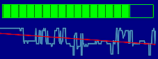
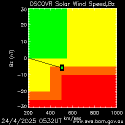

 References ↗
 Real-time propagation conditions by HF Activity Group ↗
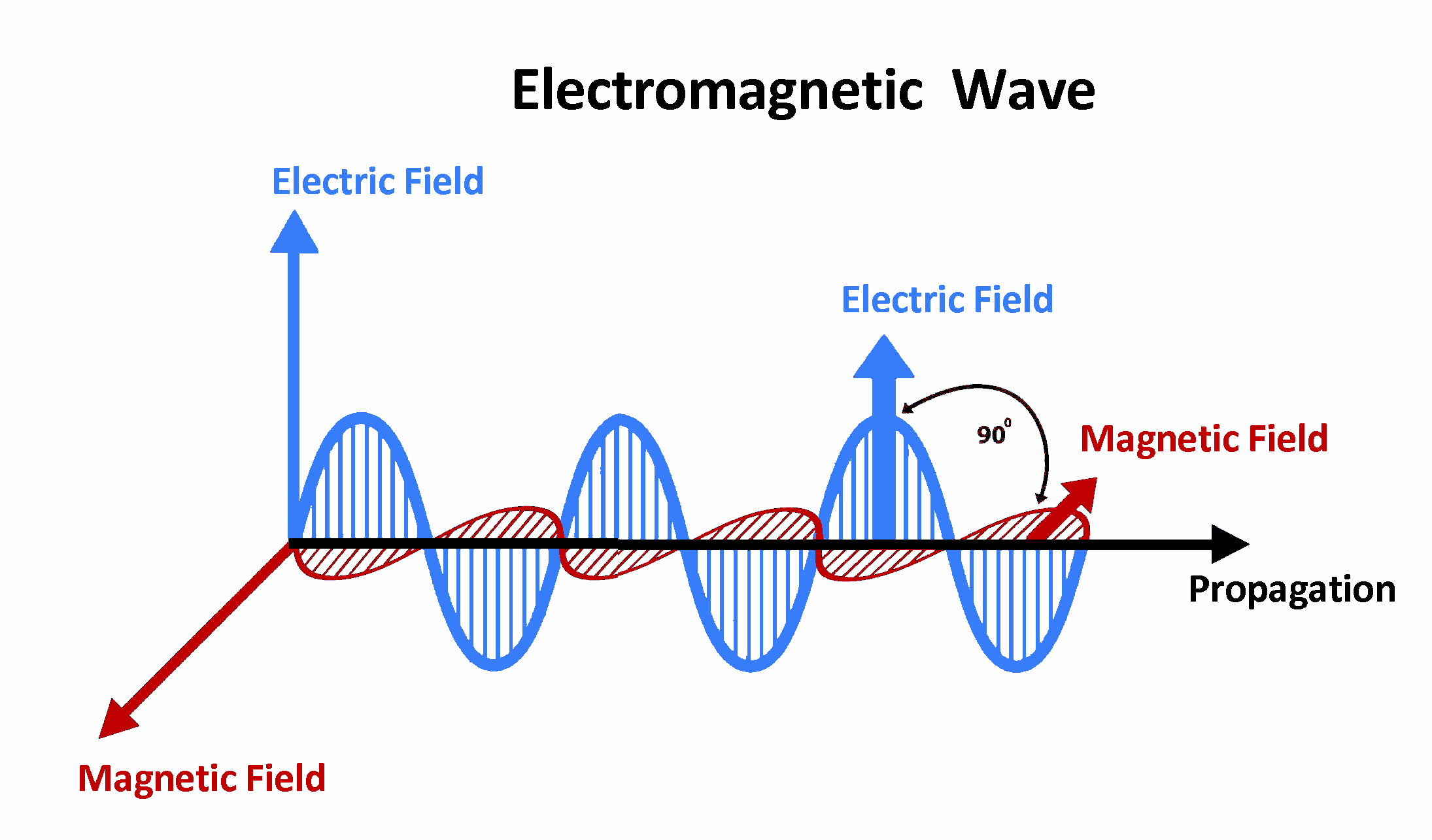
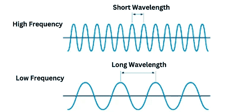

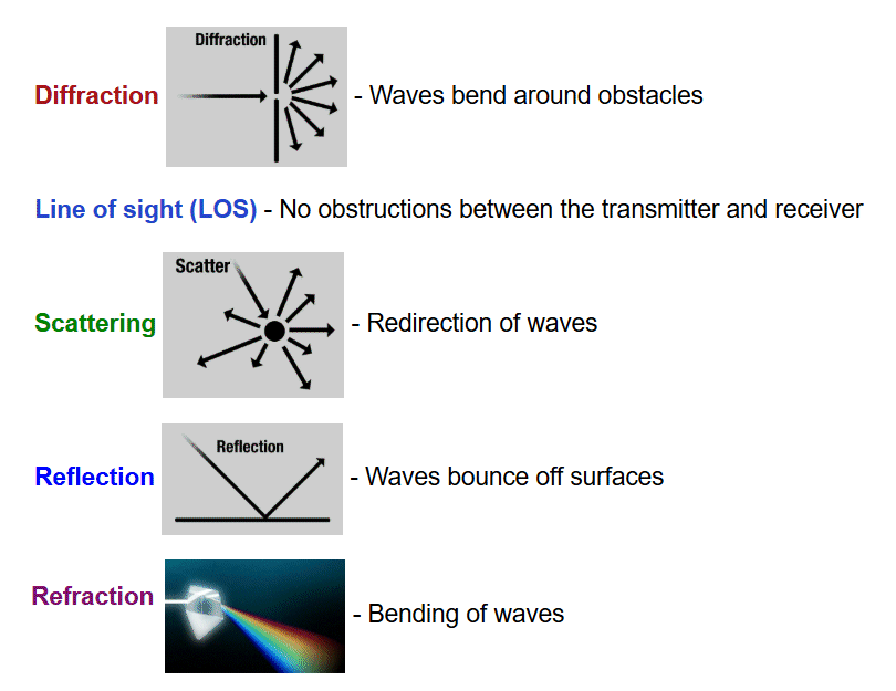
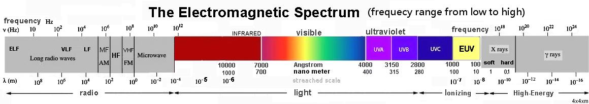
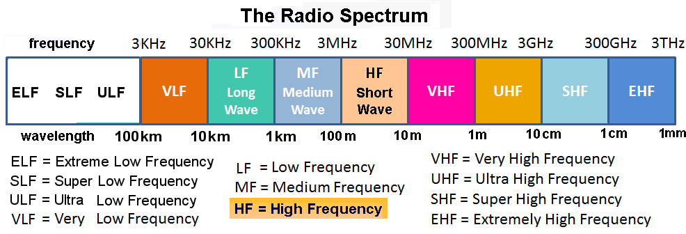
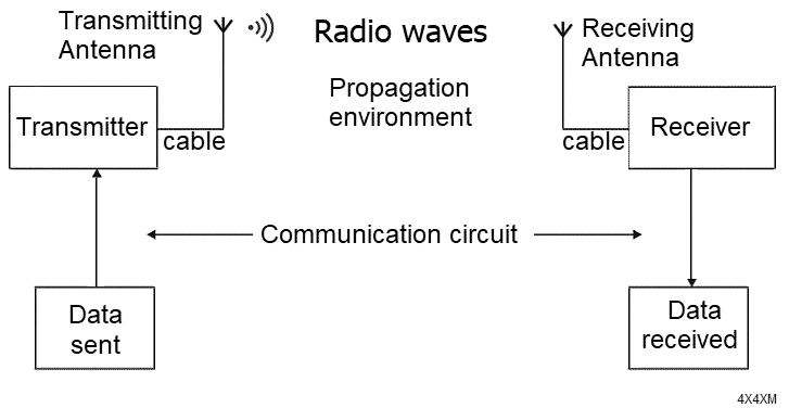


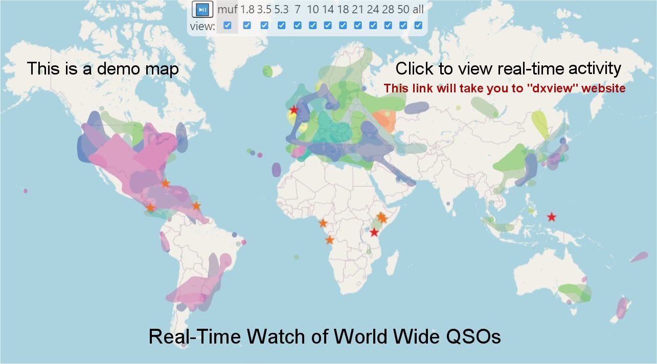
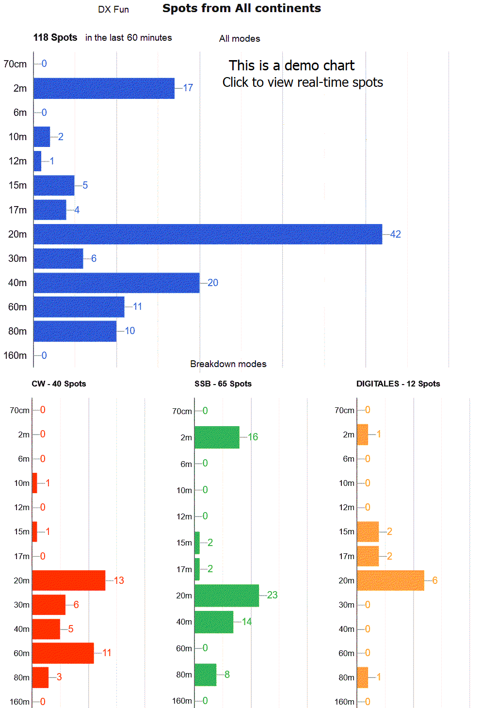
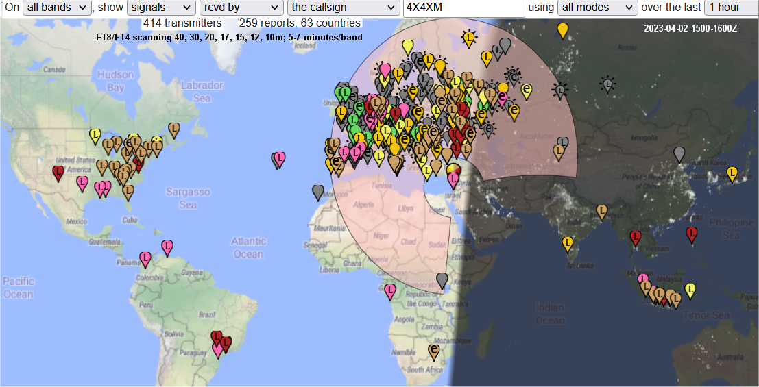
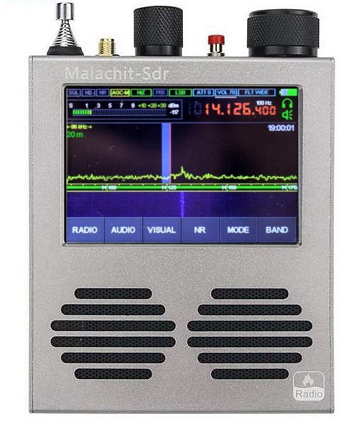

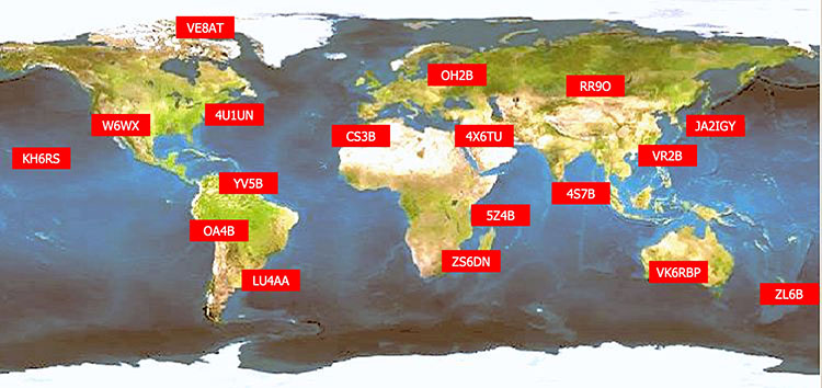
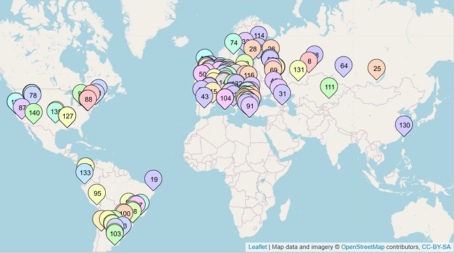
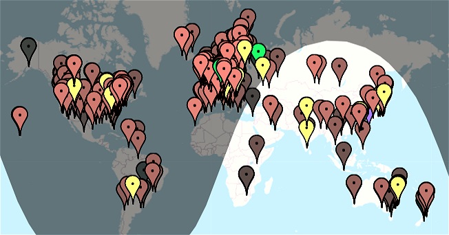
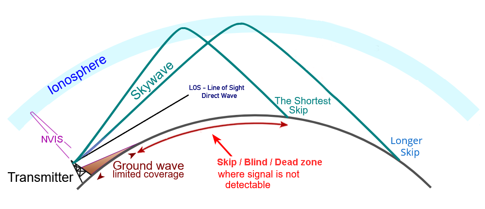
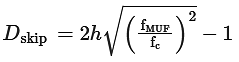
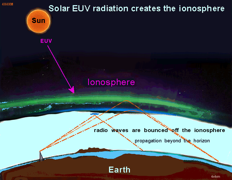


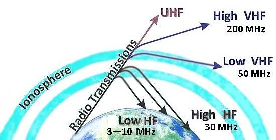

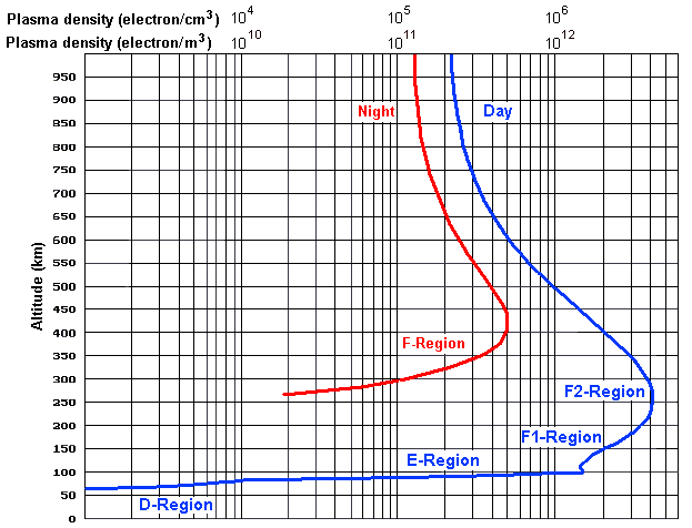
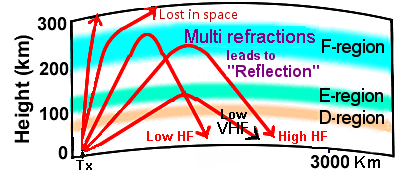


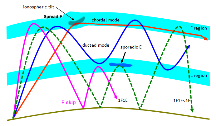

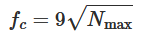 , where Nmax is the maximum electron density/m³ and fc is in Hz.
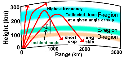


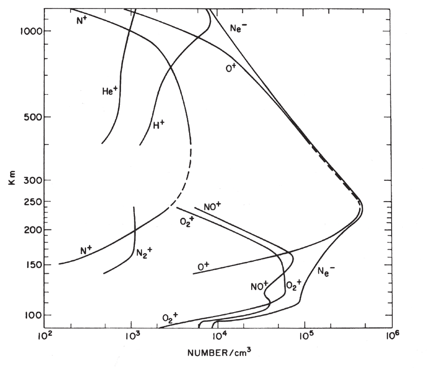
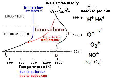
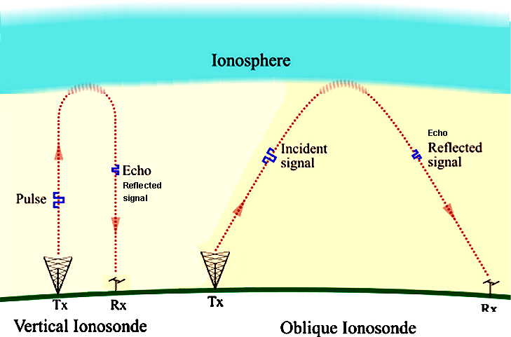


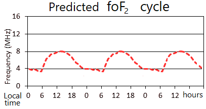


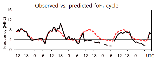
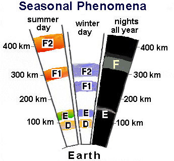
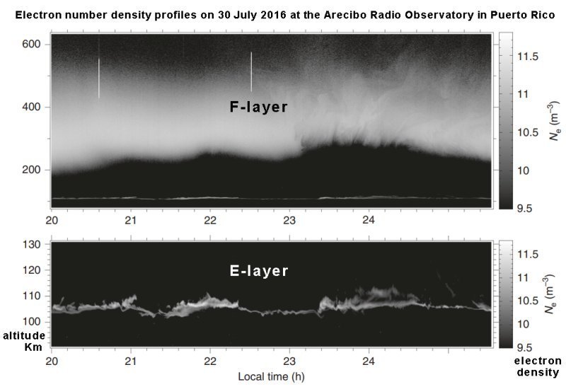


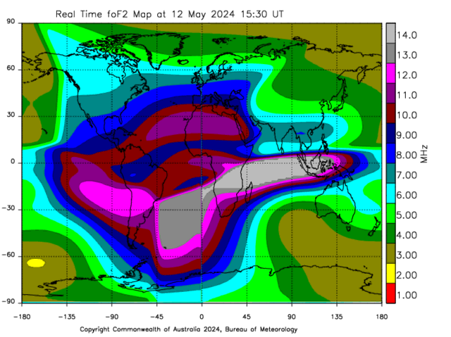
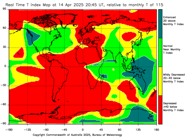
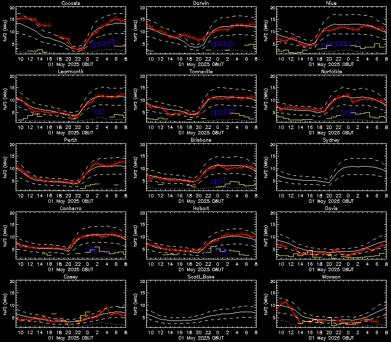
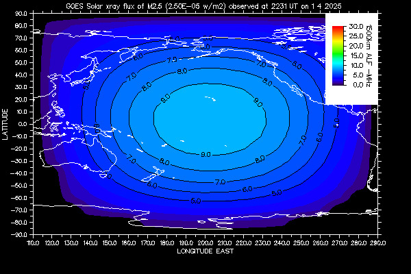
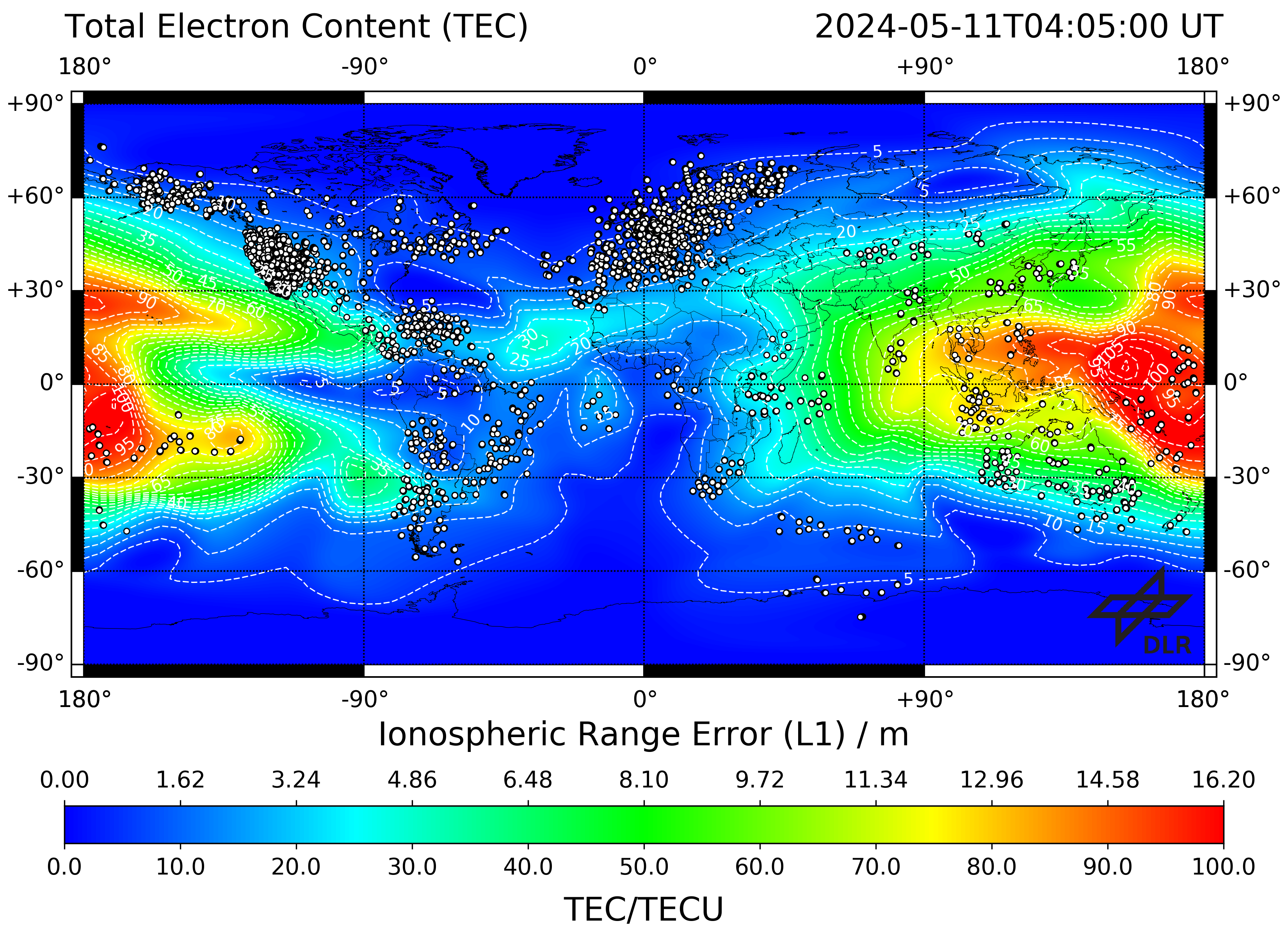


.gif)
")

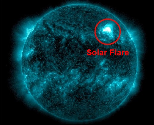
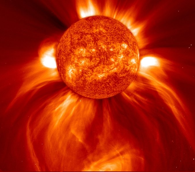
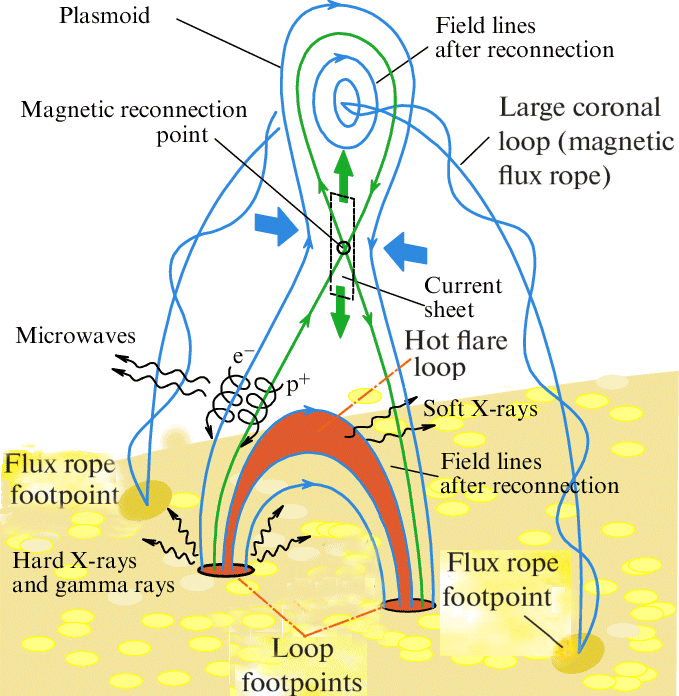


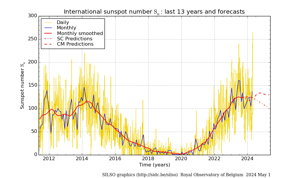
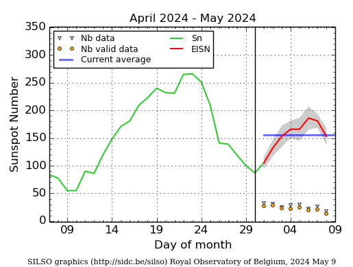
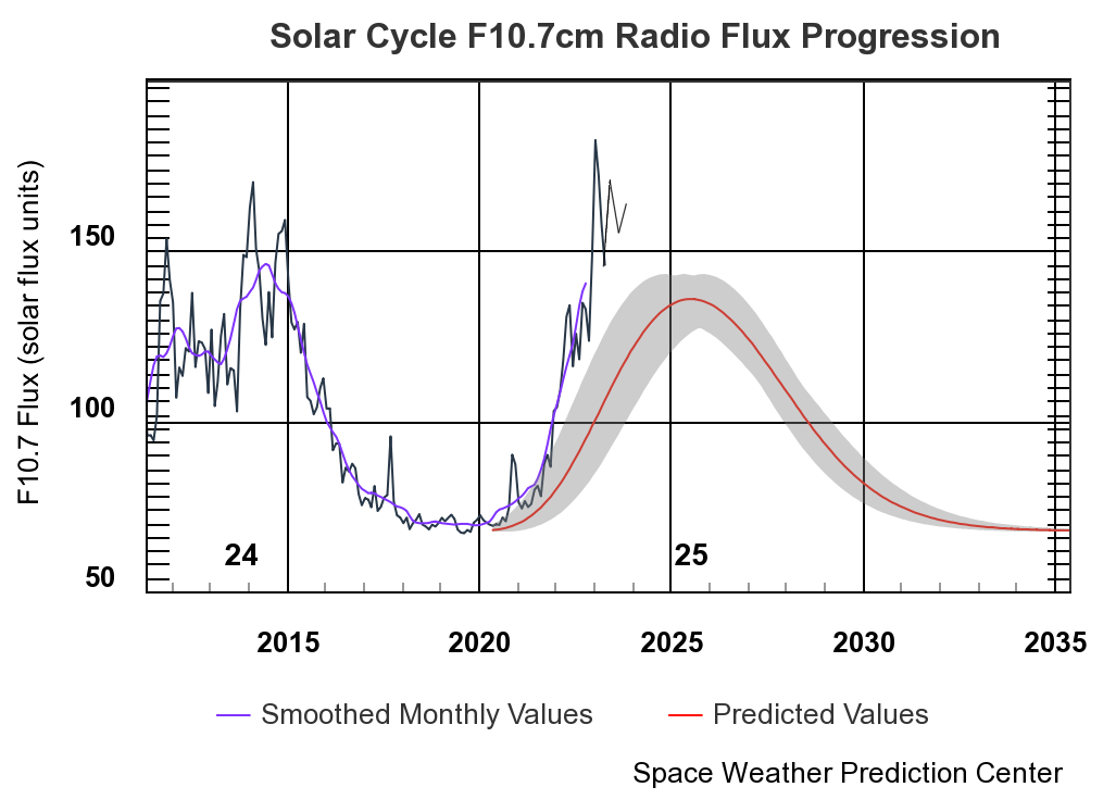
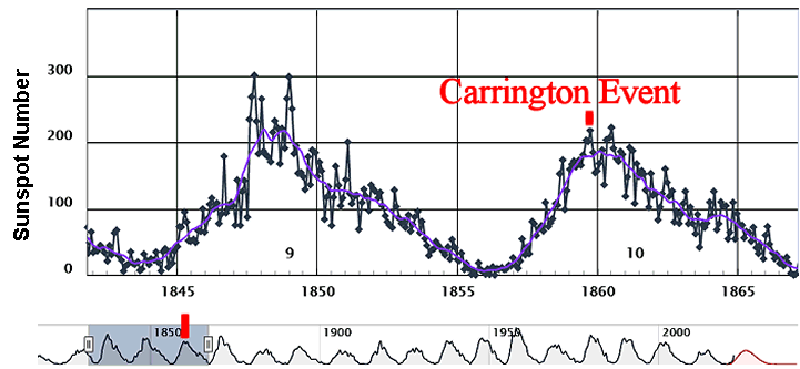
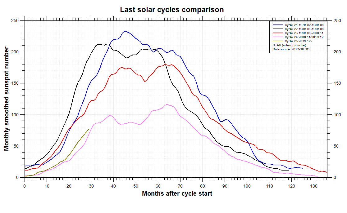


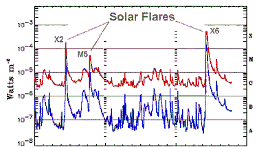
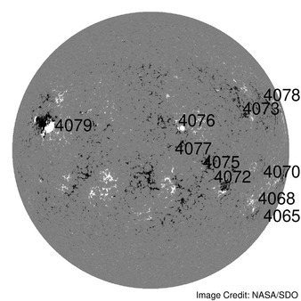
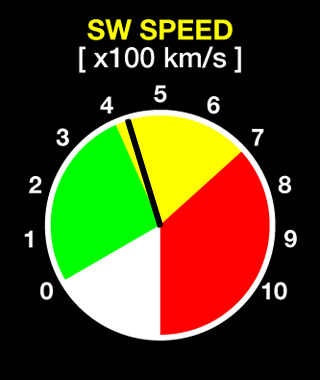

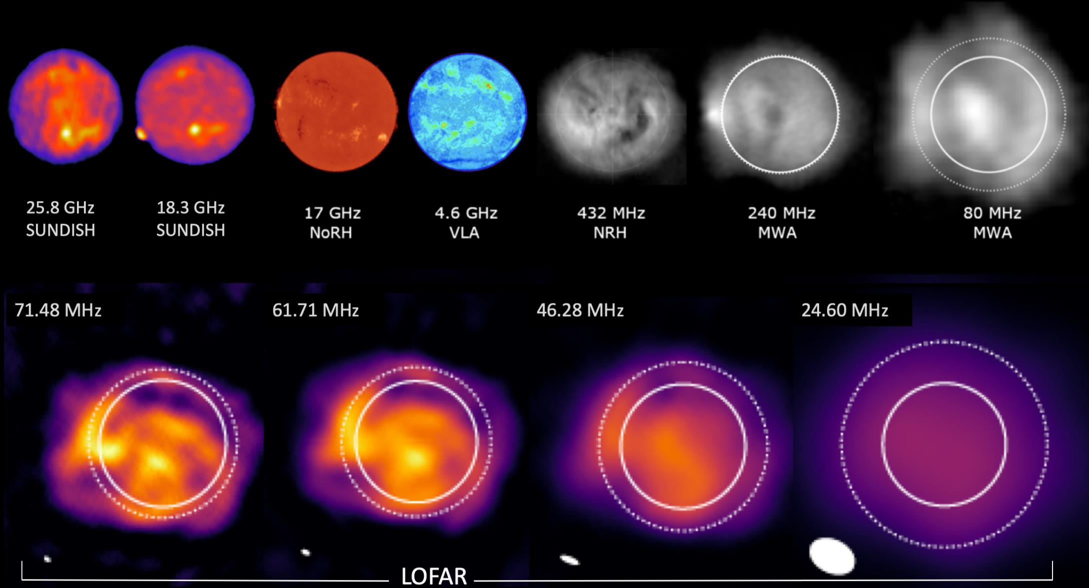
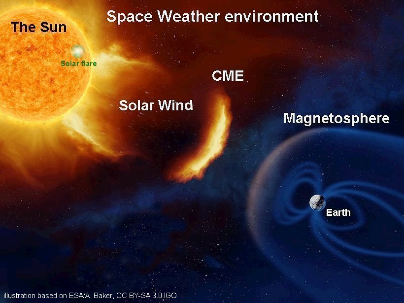
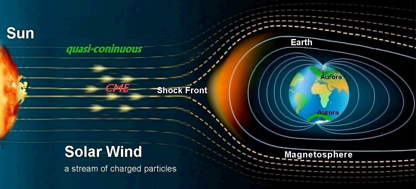
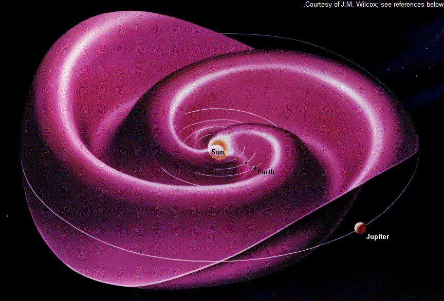
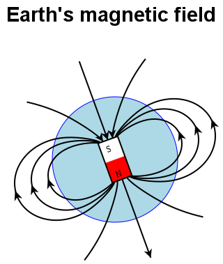
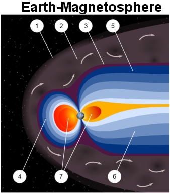
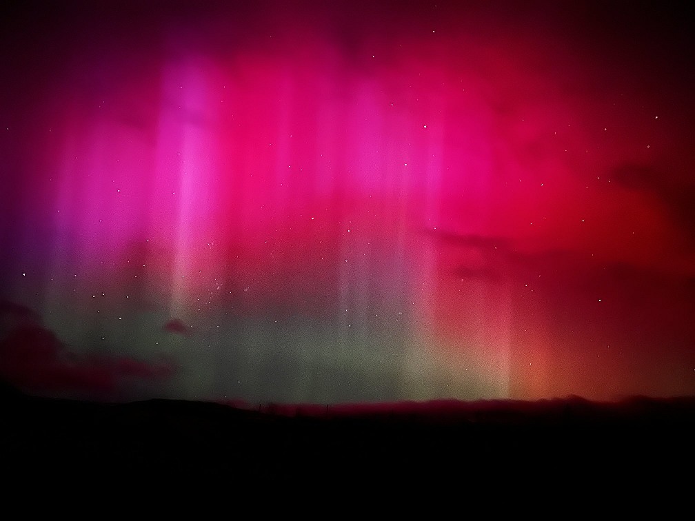
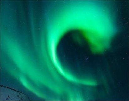
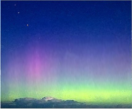

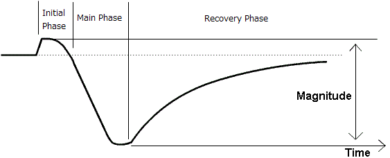


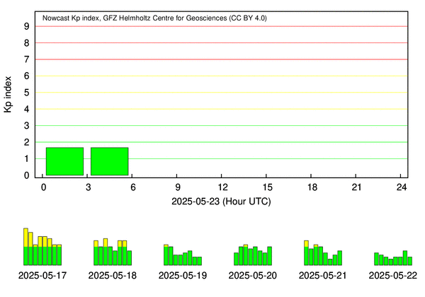
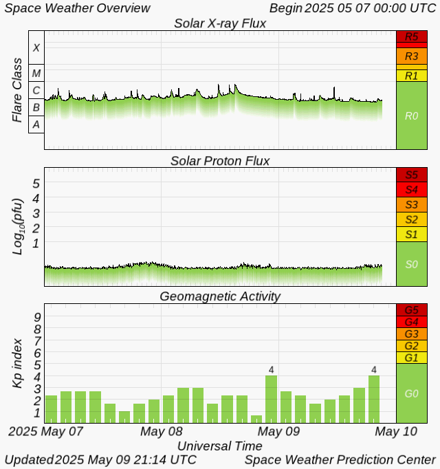


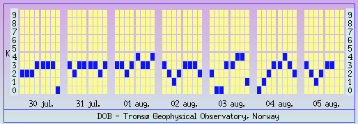
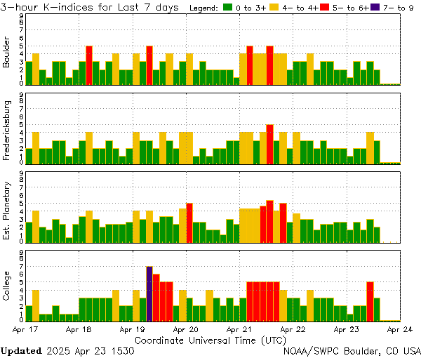
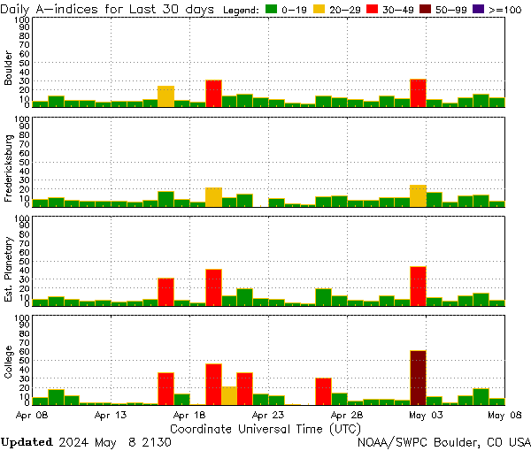
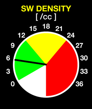
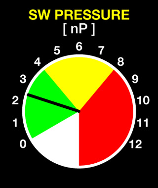
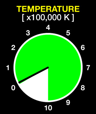
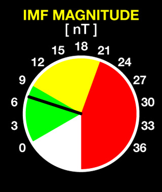
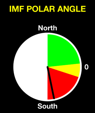
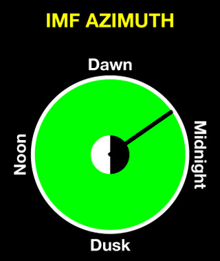
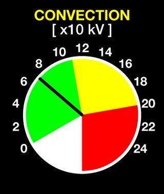
 and Alerts
  provided online by ASWPC. ↗
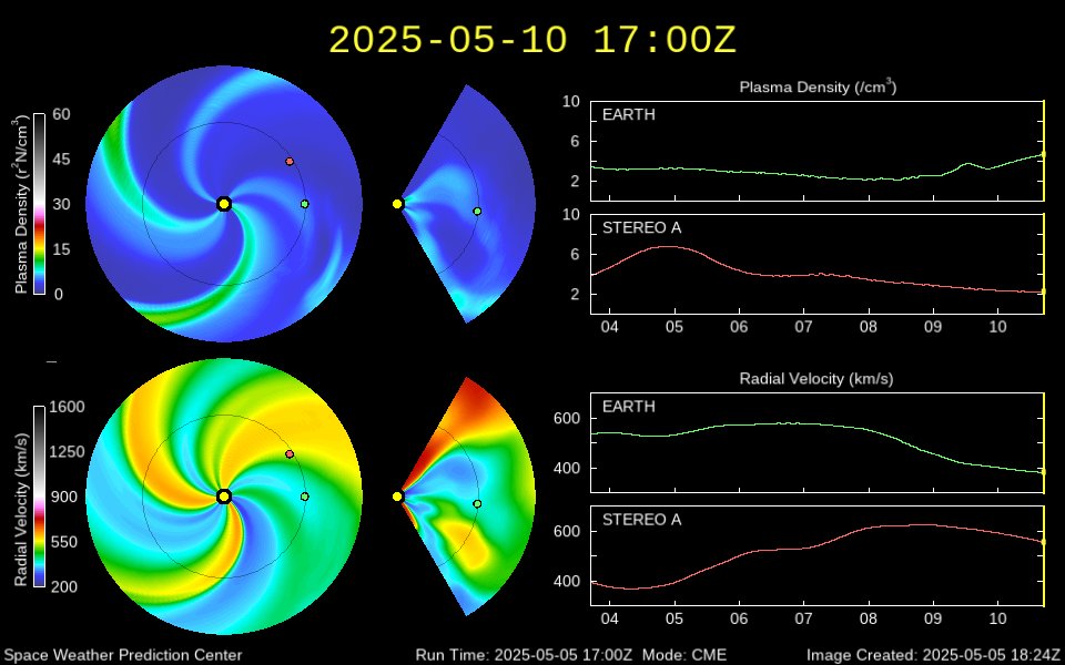
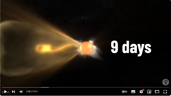
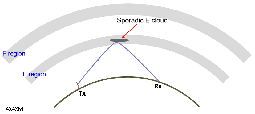


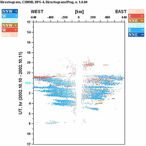
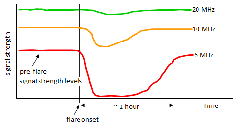
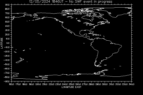
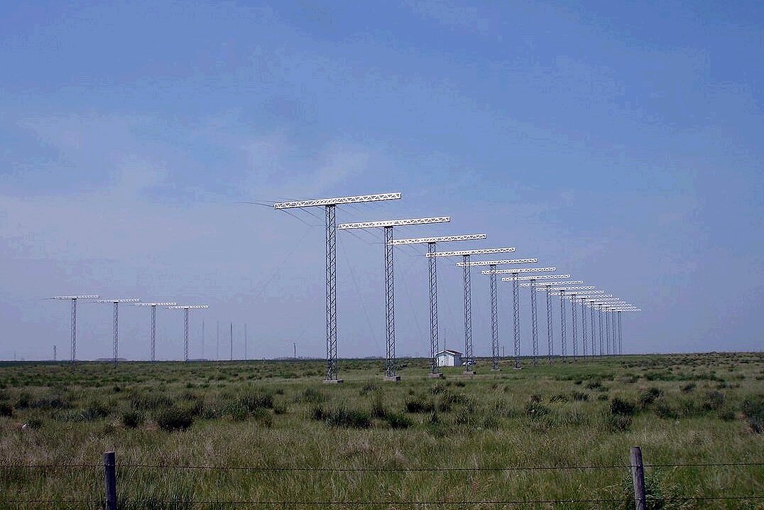
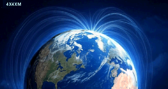


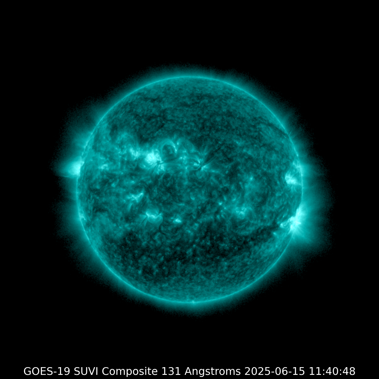
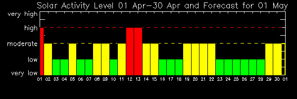
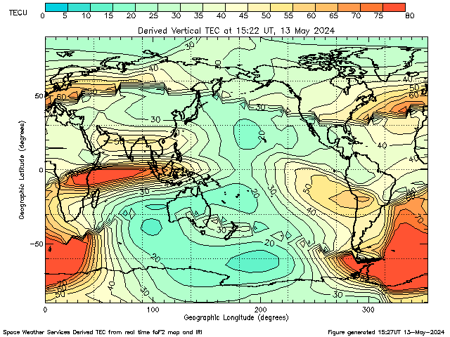
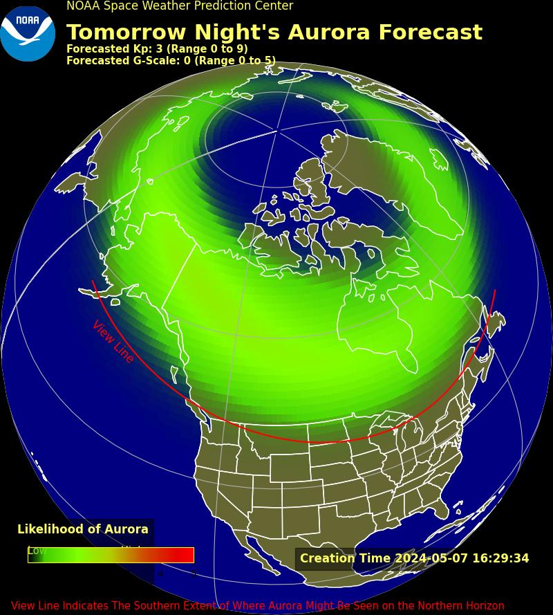