
Sample Rate- and Frequency Calibration
- always under construction -
Chapter overview
- Introduction
- One-time calibration of the sampling rate
- Continuous calibration of the sampling rate
- Continuous detection (and -possibly- correction) of a frequency offset / "drift"
-
Frequency Calibration References (Sources)
- Continuous wave (coherent) reference signals
- The Goertzel filters (to measure frequency references)
- CPU load caused by the Goertzel filters (and how to reduce it)
- The Goertzel filters (to measure frequency references)
- VLF MSK Signals as reference signals
- Periodic reference signals (like 'Alpha' / RSDN-20)
- GPS receivers with one-pulse-per-second (pps) output
- Continuous wave (coherent) reference signals
- The 'Scope' tab (local spectrum- or reference pulse display)
- The 'Debug' tab (debug messages and 'special tests')
- Interpreter Commands to control and monitor the frequency calibrators
Appendix: Soundcard clock drift measurements, Algorithm for the continuous sample rate correction , MSK Carrier Phase Detection .
See also: Spectrum Lab's main index, 'A to Z', settings, circuit window , phase- and amplitude monitors .
Introduction
This chapter is only important for phase- and precise frequency measurements, or for the detection of extremely weak but slow Morse code transmissions ('QRSS'). You don't the functions explained in this chapter for most 'normal' applications like audio frequency analysis.To improve the accuracy of frequency- and phase readings, it is possible to reduce the influence of "drifting" soundcard sample rates by permanently monitoring the frequency and phase of an external reference signal.
( This is different from the 'normal' sample rate calibration table on the audio settings screen, where the sample rate is only calibrated once but not permanently)
With the permanent frequency calibration, you can (almost) eliminate the effect of a drifting VFO in an external receiver.
Some frequency reference sources are listed in one of the following paragraphs.
One-time calibration of the sampling rate (pre-calibration)
With the following steps, you can calibrate the sampling rate once. This is enough for most applications.
- Select a nominal sample rate which is high enough to detect the "reference signal" of your choice. Most modern cards seem to work better with 48000 samples/second, rather than 44100 . These sampling rates are sufficient for most applications.
- Use a relatively high FFT resolution, for example 262144 points, in the settings for the main spectrum display.
- Make sure the spectrum/waterfall cursor readout operates in peak detecting mode.
-
With the peak-detecting cursor in the spectrum graph or the waterfall, measure
the frequency of the reference signal.
Move the mouse close to the peak frequency. The "peak indicator" circle in the spectrum plot should jump to the peak.
For example, the 'cursor' function will show a value of 15623.2345 Hz (this is an interpolated value, the resolution is much higher than the FFT bin width ! The interpolation algorithm was suggested by DF6NM, thanks Markus ... it really does an amazing job !) - Enter the "correct" and the "measured" frequency in the calibrator fields of the audio settings dialog. Then click "Calibrate". The program calculates the new sampling rate and shows it in the calibration table. If you think it's reasonable, click "Apply" to make the new value effective.
- Move the mouse to the peak of the reference signal again and check the displayed frequency (again, in 'peak'-mode). It should be very close to the true frequency of the reference signal, like 15625.0001 Hz for the "TV-sync" example.
Notes:
- The mentioned accuracy in the sub-milliHertz-region is realistic, if the soundcard in your PC has a crystal oscillator, and has been running for a few hours. If the frequency of the soundcard's oscillator drifts too fast, try the continuous calibration routine which is explained in the next chapter. Don't calibrate immediately after powering on the system - see soundcard frequency drift measurements in the appendix.
- There are different entries in the calibration table for some 'nomimal' sampling rates (like 11025, 22050, 44100, 48000, 96000 Hz). Because it is very likely that all rates are derived from the same clock oscillator, it's ok to do the calibration procedure for the highest sampling rate only, divide the calibrated result by two or four, and enter the result manually in the table. This way you can calibrate 11025 samples/second with the 15625 Hz TV sync 'indirectly'. But beware, some soundcards are known to be very far off the nominal sampling rate; most 'modern' soundcards work better at 48 kHz than at 44.1 kHz .
- In the configuration file(s), the soundcard sampling rate calibration (with nominal and true sampling rates in Hertz) are in the [SOUNDCARD] section. Each of the known 'standard' sampling rates for a soundcard has its own key name (e.g. Calib48000 for the input, and CalibOutput48000 for the output).
-
In older program versions, the SR calibration table was always saved
in the machine-depending configuration file MCONFIG.INI
in the installation directory. It was not part of a user configuration
file (SETTINGS.INI; *.USR; etc). So, if someone sends you a test setup file
via e-mail, your calibration does not get lost.
In later program versions, the SR calibration values (as well as other parameters formerly stored in MCONFIG.INI) may optionally be stored in the user configuration file (automatically saved SETTINGS.INI or user-defined filename *.USR).
It's your choice where to store the SR calibration table, controlled (from SL's main menu) via Options ... System Settings ... Filenames, Directories, and Stream I/O ... checkmark
☑ no extra file .
With 'no extra file' checked, the calibration data are stored in the *.usr file (in that case, the item text in the 'File' menu shows 'Save Settings (User + Machine) As ...'.
The sample rate calibration table is displayed in the configuration window (audio settings) under 'Audio Processing', near the selection of the 'nominal' input sampling rate. The table contains fixed entries for the most common 'soundcard' sampling rates, plus a few (3?) entries for non-standard sampling rates (marked with orange colour in the screenshot below). These entries can be used for devices like special SDRs, A/D converters, or audio streams with 'unusual' sampling rates. As often, don't forget to hit 'Apply' after manual edits in this table.

'Sample Rate Calibration Table' for inputs (e.g. ADCs) and outputs (e.g. DACs)
Note: The table columns get wider when maximizing the configuration window.
Continuous calibration of the sample rate
For 'very demanding' applications like phase measurements, or spectrograms with extreme frequency resolution (mHz or even uHz range), it may not be sufficient to "calibrate" the soundcard's sampling rate only once. Instead, the SR (sample rate) may have to be monitored continuously against a stable reference, so any SR drift can be eliminated.To achieve this, select Components ... Sampling Rate Detector from SL's main menu, or select one of the preconfigured settings (from the Quick Settings menu) which automatically activate this function (for example, the Very Slow Morse modes like "QRSS600").
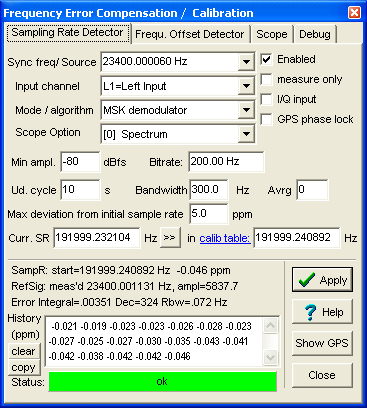
A control panel like this will open (details in a later chapter):
Control panel for the sample rate calibrator
 or
or

When selecting one of the preconfigured sources from the Sync frequency/ Source combo, the program will automatically adjust other parameters on this panel, as required. The screenshots above show a typical configuration using a VLF transmitter with MSK modulation (minimum shift keying) on the left side, and a typical configuration for a GPS receiver (with 1-pps-sync output) on the right side. The other controls on this panel are explained in a later chapter (you will usually not need to modify them, at least not if you picked one of the pre-configured references from the list).
- Note
- The 'Sync frequency / Source' combo is not just a drop-down list but also an edit field.
Click into the field to enter any frequency (below half the sampling rate, of course).
Don't forget to set the Enabled checkmark. It can be used to disable the correction temporarily (in the presence of heavy noise aka QRN). If you only want to measure your soundcard's momentary sampling rate (but not let SpecLab adjust other processing stages based on the measured sample rate), set the 'Measure Only' checkmark. If your receiver is a software defined radio with quadrature output, set the checkmark I/Q input (in that case, the Q channel will be tapped at the 'Right' input, for example L1 = Inphase, and R1 = Quadrature phase input).
After a few seconds, the SR detector has acquired enough samples to calculate the first 'true' sampling rate (see principle below if you're interested to know how it works). If the reference signal is strong enough, and a few other 'signal-valid' criteria are fulfilled, the Status field (at the bottom of the control panel) will turn green.
The 'History' in the lower part of the panel shows the sample rate's deviation (in ppm) from the nominal value, intended as an aid to compare the stability of different soundcards (the ppm values can be copied and pasted somewhere else through the windows clipboard, remember CTRL-C and CTRL-V..) . If the history shows a very 'jumpy' behaviour, the clock crystal of your soundcard may be too close to a heat source, or near a cooling fan. This may render the soundcard useless for some applications - also see soundcard drift measurements at the end of this document (it contains an example of a 'good' (low-drift) and a 'poor' (rapidly drifting) soundcard.
The proper operation of the SR detector can be monitored on the integrated 'Scope' window (not to be confused with SL's input monitors, and the time domain scope). For example, if a 'healthy' MSK signal is being received, the Scope will show something like this:
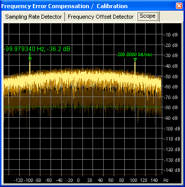
If the reference is an MSK signal, the scope shows the spectrum of the squared baseband signal. There should be two peaks in the spectrum, symmetrically around the (invisible) 'carrier frequency', spaced by the bit frequency. For example, an MSK broadcaster transmitting 200 bits per second will produce a line 100 Hz below the center frequency, and another line 100 Hz above the center. Both lines (peaks) are labelled in the scope display; one with the offset from the center, the other with the difference between both peaks in bits/second. This indicator is typically very close to the nominal bitrate (see screenshot); if not, you may be tuned to a false signal.
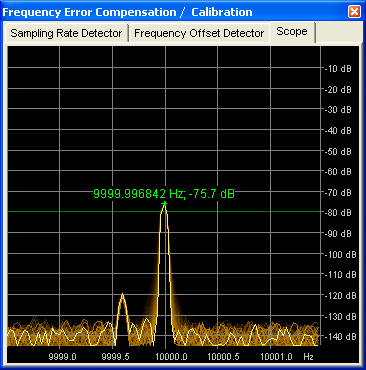
If the reference is a coherent 'carrier' (like the AM carrier of a time signal transmitter, or a longwave broadcaster), the scope will look simpler - ideally, it only shows the carrier, way above the noise level:
See also: Details about the 'scope' to monitor the operation , Settings for the sample rate calibrator, overview .
Principle
Depending on the type of the reference signal, the sample rate calibrator uses ...
-
a numerical controlled oscillator (NCO) with two outputs, 90° phase
difference ("I/Q output"),
a complex multiplier ("I/Q" mixer), the reference signal is multiplied with the NCO's outputs like in an "image cancelling zero-IF receiver",
and a chain of low-pass filters and decimators, with adjustable bandwidths. -
a bank of Goertzel filters, each filter observes
a narrow frequency band,
and emits a complex frequency bin every 10 to 30 seconds which is then processed as in the old algorithm (see details in the appendix). -
a phase meter for the decimated I/Q-samples (or the Goertzel filter with
the maximum output).
By comparing the phase in the current and the previous complex sample, the momentary frequency can be calculated with a much higher resolution than the measuring time (a few seconds) would allow in a simple 'frequency counter'. - An interpolating detector for the sync pulse from a GPS receiver (typically with a one-pulse-per-second output, aka '1 PPS'), described in a later chapter.
The phase meter produces a new reading every second (or, for the
Goertzel filters, every 10 seconds). From the difference
of phase values, the new deviation of the sampling rate is calculated, and
the 'calibrated' sampling rate (which is an input parameter for some other
function blocks) will be is slowly adjusted. Many (but not all) function
blocks in SpecLab will benefit from this 'measured' sampling rate. For example,
if the main spectrum analyser uses extremely long FFTs (with decimation)
to achieve a milli-Hertz resolution, you will need this continuous calibration.
A test showed that the clock frequency of the audio device in a notebook
PC could be 'shifted' by 1.5 ppm within half an hour, just by cooling the
notebook's underside with a fan (a 10 kHz signal was off by 15 mHz - see
soundcard clock drift in
the appendix). In many cases the permanently running sampling rate 'calibrator'
eliminates the need for an external
A/D converter (clocked with an oven-controlled or GPS-disciplined oscillator)
!
Another example: With an E-MU 0202 (external audio device capable of 192
kSamples/second), it was possible to compare the carrier phases of several
VLF transmitters, using the German DCF 77 (time signal transmitter on 77.5
kHz) as an ultra-stable frequency reference.
There are some additional function blocks in the frequency calibrator which detect the presence and the quality of the reference signal. This prevents the 'calibrated' sample rate from running away if the reference signal is bad or even missing. The 'pulling range' for the calibrated sampling rate can be adjusted by the user.
Some parts of the calibration algorithm are explained in the appendix. The monitoring display (to check if the SR detector operates properly) is explained here .
Settings for the sample rate calibrator in Spectrum Lab
There is a special control window for the sample rate detector (/compensator) in Spectrum Lab. To get there, select "View/Windows".."Sample Rate Calibrator" from Spectrum Lab's main menu, or click on the "SR calib" function block in the circuit diagram. It's not really a 'calibration', but this function allows to compensate the soundcard's sample rate drift permanently.
Controls for the 'Sample Rate Detector'
The upper part of this tabsheet controls the sampling rate detector, selects reference frequencies, source (left or right "audio" channel), and a few options on the right side of the panel shown below.
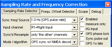
Screenshot of a part of the 'Sampling Rate Detector' panel in SL,
here configured for a GPS receiver with NMEA decoded via soundcard.
- Sync Frequency (Hz) / Reference Source :
-
The known frequency of the reference signal (as it should be).
Please note that the sample rate detector uses audio, or "baseband" frequencies
but not "radio" frequency. A number of predefined
frequency references can be picked from this list, too. Picking one of
the references from the list may automatically change some other parameters
(like the mode/algorithm field) . For example, selecting "GPS, 1 pps" from
the list will automatically set the 'Mode/algorithm' to 'GPS sync with NMEA
decoder' (see below).
- Input Channel
-
Defines where the reference signal is taken from. Choices are 'LEFT input'
or 'RIGHT input' if the program runs in stereo mode. For I/Q input, the
'quadrature' component (Q) will be the complementary channel, for example
I=L1, Q=R1, etc.
- Synchronized Resampling
-
If this option is activated, the SR detector will be closely tied
to Spectrum Lab's Input Preprocessor:
The SR detector continuously measures the current sampling rate from the input device ("soundcard"), and the preprocessor's resampler converts the stream into a sequence with exactly the nominal sampling rate. For example, even if the soundcard's sampling rate drifts around between 47990 and 48001 samples per second, the output (from the preprocessor to labels 'L1' and/or 'R1' in the circuit window) will be 48000.000 samples / second, depending on the quality of the reference.
If there are two active input channels (labelled L0/R0 in the circuit diagram), the combination of 'Input Channel' and 'Synchronized Resampling' affects which of the two channels is routed from L0/R0 to L1/R1 :- 'Input channel' for the calibrator = R0
'Synchronized Resampling' = "only 'the other' channel(s)" - R0 (right audio channel) delivers NMEA and sync pulse from the GPS.
L0 (left audio channel) delivers, for example, a VLF signal.
This is the combination used when the screenshot of the circuit window (below) was made;
and it's the method of choice for the amateur VLF-BPSK experiments in 2015.

Screenshot of the A/D converter block connected to SL's input preprocessor.
'L0' = left channel, directly from the soundcard, here approximately 192 kSamples/second;
'R0' = right channel, directly from the soundcard, feeds GPS sync+NMEA into the calibrator.
'L1' = output from preprocessor to the rest of the circuit with exactly 48 kS/s;
'R1': not connected due to the configuration of the Sampling Rate Detector (!)
- 'Input channel' for the calibrator = R0
'Synchronized Resampling' = "all channels" - Both inputs (L0 and R0) run through the resampler to bring their sampling to the nominal value. Quite useless for GPS-sync, but makes perfect sense for other references (like MSK transmitters on 'the same band' or 'on the same antenna' as the measured signal).
- 'Input channel' for the calibrator = R0
'Synchronized Resampling' = "all input channels" - Both inputs (L0 and R0) run through the resampler
to bring their sampling to the nominal value (routed to L1 and R1).
Quite useless for GPS-sync, but makes perfect sense for other references (like MSK transmitters on 'the same band' or 'on the same antenna' as the measured signal). - 'Input channel' for the calibrator = R0
'Synchronized Resampling' = "none (don't resample)" - L0 is directly connected to L1, and R0 is directly connected to R1,
because nothing is resampled (at least not within the preprocessor).
The sampling rate is continuously measured but not corrected by resampling.
- 'Input channel' for the calibrator = R0
- Mode / algorithm
-
Allows to switch between the 'old' algorithm (which is basically a phase
meter for the reference signal), the Goertzel filters,
the MSK demodulator, and the
GPS sync pulse /
NMEA decoder. The 'mode' setting
also affects the Scope display.
- Enabled
-
Must be checked to activate the sample rate calibrator .
- Measure Only
-
Used during development or for "testing purposes". If this checkbox is marked,
the sample rate is measured, but the other components in Spectrum Lab are
not affected (they keep using the constant 'calibrated' sample rate from
the table on the audio settings panel).
- I/Q Input
-
May only be set if the signal source uses in-phase and quadrature, which
is often the case with software defined radios and similar downconverters
with complex output.
- GPS phase lock
-
This highly experimental option can only be used if the reference (source)
is a GPS receiver with sync pulse output (pps). When checked, all oscillators,
sinewave generators, etc inside the software don't use the number of samples
acquired from the soundcard as argument, but the precise time of day from
the GPS receiver's NMEA- and sync output. The phases of most oscillator outputs
will then be phase-locked to the GPS sync pulse. At midnight (precisely,
at 00:00:00.0000 'GPS time', which is close to UTC), all circuit components
which can be 'locked' to GPS this way (see list below) will reset their phase
angles (or sine wave arguments) to zero. Such phase jumps do not occurr if
the oscillator frequency is an integer multiple of 1 Hz / ( 24 * 60 * 60
) . If the frequency is an integer value (i.e. a multiple of 1.0 Hz),
there will be no phase jump, and the phase noise may be slightly less than
at arbitrary frequencies.
Circuit components affected by this option are :
- The sine wave outputs in the Test Signal Generator (unless they are frequency modulated)
- Most (but unfortunately not all yet) of the digimode encoders (PSK, FSK, ASK,..)
- The 'oscillators' for frequency shifters ('mixers') before the main analyser's FFT, when configured for "Complex input with internal frequency shift".
- GPS 1s late ("GPS / NMEA output one second late")
- Only has an effect in mode 'GPS sync with NMEA decoder'. If the GPS-based timestamps
are one second late, set this option.
For details, see Checking the GPS NMEA timing'.
- Min. Reference Amplitude
-
If the strength of the reference signal is less than this value, the sample
rate calibration will be temporarily disabled (important if you use 15625
Hz as reference and someone turns the TV off !). A typical value is -80 dBfs,
wich means "80 dB below the maximum level which can be handled by the ADC).
Keep the amplitude of the reference signal as low as possible (typically
about -60 dBfs) to leave enough headroom for other signals you want to
measure.
The current (measured) signal strength is displayed in the lower part of the control window.
- Periodicity
-
Rarely used, and only works with the Goertzel option. The only known use
was for the Russian 'Alpha' VLF transmitters,
which do not send a continuous signal but a periodic sequence which repeats
0.2777777 times each seconds.
This periodicity causes multiple spectral lines (separated 0.2777777 Hz from each other), which the calibrator must know to avoid 'locking' on the false line (because the strongest 'Alpha' line is not always the one with the nominal frequency). If you pick one of the 'Alpha' frequencies in the Reference Frequency list, the Periodicity field (in Hz) will be automatically filled. For normal (continuous wave) reference signals, leave this field empty.
If the mode is set to GPS sync / NMEA, the periodicy field is used to enter the serial bitrate of the GPS receiver's NMEA output, which is important for decoding the GPS time.
- Update Cycle :
-
Number of seconds per measuring interval. Longer intervals (10 or even 30
seconds) are preferred because they allow frequency measurements with better
accuracy. On the other hand, if the soundcard's sampling rate drifts rapidly
(as can often be seen with internal soundcards), shorter intervals (less
than 10 seconds) can give better results, because even "short excursions"
of the sampling rate will be compensated.
- Observed Bandwidth
-
Defines the width of the frequency window for the sample rate. A typical
value is 0.5 Hz (for a 15625 Hz reference). If the bandwidth is too low,
the phase meter may not "see" the reference signal if the sample rate is
too far off. If the bandwidth is set too high, the phase meter gets less
immune to noise. If a the calibrator uses a bank of Goertzel filters (to
observe the band), the CPU load depends on the observed bandwidth, because
the larger the bandwidth, the more Goertzel filters must run in parallel
(each Goertzel filter has a bandwidth of approximately 0.1 Hz).
- Max. offset (from calibrated sample rate)
-
The initial value for the ADC's sample rate is taken from a table in SpecLab's
'audio settings'. The deviation
between the sample rate in the table and the result of the calibration procedure
must not exceed a certain value, like this:
Sample Rate from calibration table in the 'audio settings': 44103 Hz
Max Deviation: 5 ppm -> true calibrated sample rate = 44103 Hz +/- 5 ppm = 44103 +/- 0.2 Hz = 44102.8 .. .44103.2 Hz.
(Note: this has nothing to do with the 'nominal sample rate' 44100 Hz, so you should do a first 'coarse' calibration for your soundcard before activating this function. The reason why only a small 'deviation' range should be used is to have a good starting value for the narrow-band phase meter. )
A typical soundcard oscillator drift, after booting up a "cold" PC, can be found in the appendix . For PCs operated indoors, or at a relatively 'constant' temperature, 5 ppm should be sufficient.
- Current sample rate
-
Displays the currently calculated sample rate. You cannot edit this field,
but copy its contents into the clipboard. Mark the text with the mouse and
press CTRL-C to copy into the windows clipboard. You can then insert the
copied value as a "very good starting point" into the calibration table in
SpecLab's audio settings screen.
Values displayed on 'Sample Rate Detector' control panel
Depending on the mode / algorithm settings ( phase meter / MSK demodulator / Goertzel filters), the following values may be displayed on the SR detector's control panel :
- SampR : start = <freq> Hz + / - <dev> ppm
-
Shows the initial sampling rate (usually taken from the 'calibration' table
on the audio settings panel), and the currently measured offset in ppm (parts
per million).
- Reference signal strength, quality, and / or currently measured frequency :
-
If the 'simple phase meter' is used, this line shows the signal strength
after narrow-band filtering and the signal to signal-plus-noise ratio ( "S/(S+N)"
). The S/(S+N) value compares the amplitude of the narrow-band filtered value
against a medium-bandwidth value, usually ten times the narrow-band value.
If the Goertzel filters (DFT) is used, this line shows the frequency of the reference signal (i.e. the "strongest peak" in the observed frequency range), and the signal strength in dBfs (dB "over full scale", thus always negative).
- Error Integral (only active when using the Goertzel filters) :
-
Shows the summed-up products of frequency difference ("measured" sampling
rate minus "predicted" sampling rate) from each measuring cycle, multiplied
by the measuring interval time in seconds. Thus the unit of this 'integral'
has no unit (it can be considered Hertz * seconds, though). If the sampling
rate doesn't drift at all, or drifts at a constant, linear rate, the "predicted"
sample rate (for the end of the next measuring cycle) will be equal to the
"measured" sampling rate, and the SR Error Integral will be zero.
Note: Long-term phase observations (for ionospheric studies, etc; using the pam function) only make sense if the error integral stays almost zero; i.e. the drift must be very low or at least predictable. Internal soundcards are usually not suited for such long-term phase measurements, but some external audio devices (especially USB devices in "large boxes") are.
Internally, the a fraction of the error integral is used to steer the 'predicted sampling rate' (until the end of the next measuring cycle) to minimize slow drifting effects in long-term phase measurements. The error integral can be reset (cleared) by clicking the 'Apply' button on the Sample Rate Detector panel - it simply restarts the detector, which includes "forgetting" old values.
- Rbw: Receiver Bandwidth (in Hertz)
-
Depends on the mode, but is usually dictated by the
update cycle .
- Decimation (only displayed when the calibrator uses a narrow-band reference signal) :
-
Shows the scheme how the high audio sample rate and ADC bandwidth (like 44100
samples/second and 22050 Hz bandwidth) is reduced in chain of decimator stages
down to the phase meter's sample rate and bandwidth (like 1 sample/second
and 0.5 Hz bandwidth). Every decimator stage can reduce sample rate and bandwidth
either by 2 or by 3, the total decimation ratio is also shown here. With
a large decimation ratio, you can use signals buried in the noise as reference
!
- Phase angle (only displayed when the calibrator measures the phase of a reference signal) :
-
Shows the actual value of the phase meter (reference
signal - oscillator). The displayed value should be constant, only
a small phase jitter is unavoidable (usually below 0.5 °).
- System time minus GPS time (only displayed in the 'GPS sync' modes) :
-
Shows the current difference between the PC's internal system time and the time extracted
from the GPS data (sync pulse and NMEA if possible).
If only the GPS sync pulse ("PPS" signal) is connected, but not the NMEA data output, the integer part of the time difference is meaningless because in that case, Spectrum Lab can only "guess" the GPS time.
If only the PPS signal is connected, the fractional part of the time difference must be well below 500 milliseconds. The same value can be retrieved via interpreter function sr_cal.systimediff . - Status:
-
If this panel is green, everything is ok; otherwise the text shows what may
be wrong, for example:
"SR range exceeded"
"S/(S+N) ratio too bad"
"Reference signal too weak", etc.
Continuous detection (+"calibration?") of a frequency offset
The frequency offset detector works similar like the sample rate detector (see previous chapter). The result from the frequency measurement is not used to determine the (corrected) sample rate. Instead, the frequency difference (deviation) between a reference frequency and the measured frequency is calculated. This can be used to...
- compensate a slowly drifting oscillator in an external receiver
- measure small changes in the frequency between a well-known "reference" signal and an unknown "received" signal
- correct the frequency error for the display by subtracting it from the frequency shift for the complex FFT.
- steer the VFO (in SpecLab's test circuit) to compensate the offset in the time domain
(Note: The detection of the soundcard's sampling rate AND the frequency offset detector can run simultaneously, but you need two different reference signals then. For example: one reference signal at 15.625 kHz to "calibrate" the sampling rate, and another like 1000 Hz to detect the frequency drift in your shortwave receiver. To calibrate your receiver, the 2nd reference signal must be produced in your receiver, of course. Details below).
To activate the frequency offset detector from SpecLab's main menu, select
"View/Windows" ... "Frequency Offset Detector".
A small control window opens, where the following parameters can be set:
- Enabled:
-
Must be checked to start the F.O. calibrator.
- Source channel:
-
Select the LEFT or RIGHT input channel of the soundcard (unlike other function
blocks in SpecLab, this one cannot be connected to any signal in the
signal processing chain !).
If the input (into SpecLab) is a complex aka "I/Q"-signal, set the source to "BOTH inputs (complex)". In that case the frequency offset detector can process positive as well as negative input frequencies.
- Reference Frequency (Hz):
-
The known frequency of the reference signal (as it should be).
Please note that the frequency offset detector uses audio, or "baseband"
frequencies but not "radio" frequency. So, in this field, enter the AUDIO
(or "downconverted") frequency. A number of
predefined frequency references can be picked
from this list, too. Picking one of the references from the list may
automatically change some other parameters (like the mode/algorithm field)
.
- Min Reference Amplitude (dB):
-
The detector will be passive if the amplitude of the reference signal is
below this value. This prevents "running away" if the reference fails.
- Max Offset (Hz):
-
This is the maximum "pulling range" for the detector. In most cases, this
field will be set to the same value as the "observed bandwidth" below.
- Observed bandwidth (Hz):
-
This is the bandwidth of phase meter (which is used internally used to measure
the frequency offset; unless the Goertzel filters are in use). If your receiver
may be "off" by +/-0.5 Hz, set the 'observed bandwidth' to 1.0 (!) Hz. Otherwise
the detector may not be able to "see" the initial frequency of the reference
signal and never lock on it.
- Actual Peak Frequency:
-
Shows the "main peak frequency" within the detector's bandwidth. Can be used
for high-precision frequency measurements, but depends a bit on the signal/noise
ratio (within the detector's bandwidth).
- Averages:
-
Can be used to suppress unstable reference signals, and reduce the effect
of pulse-type noise. "50" means, the "average offset value" is calculated
from the last 50 values from the phase meter. Practical values are 50...200.
If the displayed average frequency offset appears to be "too noisy" (see
below), increase the number of averages. If the detector reacts too slow,
reduce this number.
- Avrg Offset:
-
Shows the current output of the detector, which can optionally be used to
enhance the accuracy of the main spectrum analyser (when running in "complex
FFT mode with frequency shift"), and in the time domain scope (when used
as a "phase meter"). The frequency error measured with the frequency offset
detector can be "subtracted" by the local oscillator which sets the "center
frequency" of the FFT and the scope's phase meter.
In the lower part of the window, some other values are displayed which were used during program development. One of them is the "signal / (signal+noise)" ratio, which is a crude indicator for the reference signal's quality. If the quality is very poor, the "result" of the frequency offset detector freezes, and the detector's "status" indicator turns yellow or even red (which can also be seem on the circuit window).
RED = "Reference signal too weak"
YELLOW = "Signal to noise ratio of reference signal too bad"
To calibrate a drifting receiver, you must find a way to feed a add a weak but very stable reference signal to the antenna input, which produces a suitable audio tone in the output. Use your imagination - and an oven controlled crystal oscillator, and a chain of dividers/multipliers, or a programmable DDS generator.
Frequency References
The following list contains a few frequency reference sources which can be used by SL to measure the sample rate. Some of them are listed in the 'Reference Frequency' combo of the sample rate calibrator, so you don't need to type in the frequencies yourself.
- The 1-pulse-per-second output of a good GPS receiver (jitter less than a microsecond). Since SL V2.76, receivers with 1 pps are directly supported (no need to lock to a 'harmonic' for these signals anymore). Details on using a GPS receiver with pps output follows in a later chapter. BTW, using a GPS receiver (especially such a sensitive one like the Garmin GPS18x LVC) is now the author's first choice.
- The output from an ovenned crystal oscillator (OCXO), divided down into the audio frequency range. Such 'large canned oscillators' can be found on hamfests or auctions, since they are widely used in wireless communication equipment. 5 or 10 MHz are common frequencies for such oscillators.
- The divided-down carrier frequency of a longwave time-code transmitter like MSF (60kHz), DCF77 (77.5kHz), or similar. Use a PLL cuircuit to recover a 'clean' carrier signal, then (for example) divide 77.5kHz by 31 or 60kHz by 24. The result should be a very stable 2500 Hz signal which can be fed into the soundcard. If you have a soundcard which supports 192 kHz sampling, you don't need any hardware because the soundcard should be able to receive 77.5 kHz directly with a few meters of wire.
- Some Navy transmitters in the VLF spectrum (17 to 24 kHz, or up to 90 kHz if the soundcard permits) can be used as a reference signal, if they use MSK modulation(minimum shift keying).
- Some longwave broadcasters (like the BBC's Droitwich transmitter on 198 kHz) use Rubidium standards for their carrier signal. In western europe, use a simple PLL oscillator, and divide the signal down with a cheap CMOS circuit (only required if you don't use a software defined radio like SDR-IQ or Perseus, which can be tuned to any frequency in the LF, MF, or HF spectrum).
- Any of the Russian 'Alpha' (aka RSDN-20) VLF transmitters on 11 to 14 kHz; their exact frequencies can be picked from the 'reference frequencies' combo. When doing that, the 'Periodicity' field will automatically be set to 0.277777 Hz (= the repetition frequency of the "beeps", 1 / 3.6 seconds). Some details on using the Alpha beacons as a frequency reference can be found in the chapter about the Goertzel-filter-based calibrator.
-
The line sync signal of some TV broadcasting stations.
In EUROPE (and, most likely, countries with 50 Hz AC mains): Frequency exactly 15625 Hz. While we still had terrestrial "analog" TV transmitters, the german "ZDF" derived their TV sync signals from a high-precision standard clock.
In the US (and other countries using 60 Hz AC mains), the line sync frequency is ideally 15734.2657343 Hz (for NTSC, colour, 4.5 MHz sound subcarrier divided by 286).
Update: It is questionable if the TV sync frequency still has this precision, now that everything (in Europe, even terrestrial transmissions) are digital. The sync frequencies *may* be generated by a cheap computer-grade crystal in the set-top box of your TV, so in case of doubt use one of the other sources... preferrably a GPS receiver with PPS output. -
The stereo pilot tone of a few FM broadcasting stations.Not many FM stations have their 19 kHz pilot tone locked to an atomic clock, at least not in Germany. - Any other reference can be used, as long as it can be processed with the audio card. If the ADC supports a sample rate of 44100 Hz, the reference signal can be everything between 16 Hz ... 22 kHz.
Continuous wave (coherent) reference signals
Goertzel Filters (to measure frequency references)
Depending on the checkmark 'use Goertzel' on the configuration tab, a bank of Goertzel filters is used to calculate a complex DFT (discrete fourier transform) over a narrow frequency range. Each filter measures a frequency for 30 seconds, with a frequency bin width of approximately 0.033 Hz (the effective bandwidth is a bit more due to the Hann window).
One of the Goertzel filters will (hopefully) catch the 'peak' of the reference signal - ideally in the center frequency bin. The phase angle in the output of the filter with the maximum amplitude will be compared with the previous value (from the same frequency bin). This phase difference (between the most recent and the previous complex value) is used to measure the intantaneous frequency of the reference signal, with a much higher resolution than the DFT's frequency bin width (which, as noted above, is about 0.1 Hz). Along with the phase angle, the program can determine the frequency to a few micro-Hertz (!) even though the measuring interval is only 10 seconds.
-
The result of this calculation, along with the narrow-band spectrum of the
observed frequency range, is displayed on the 'Scope' tab in the Sample Rate
Calibrator window.
Displaying the 'measured' frequency with so many digits is usually 'overkill', but it helps to check devices with oven-controlled or temperature compensated oscillators. But the reference signal must have a very good SNR (like the signal in the screenshot below) for the micro-Hertz digit to be useful. The device under test was an E-MU 0202 at 48000 samples/s .
CPU load caused by the Goertzel filters (and how to reduce it)
Depending on how the calibrator is configured, it may cause a significant extra CPU load on your system. For example, if the sample rate calibrator shall observe a 1.5 Hz wide band with 33 mHz resolution (per frequency bin), there will be 45 (!) Goertzel filters running in parallel, each at 48 kSamples/second. On a 1.6 GHz Centrino CPU, this example used 12 % CPU time (from one CPU).
Fortunately, in a normal environment, the soundcard's oscillator will drift
less than one ppm (parts per million) after warm-up, so you will get along
with a much smaller 'observed bandwidth' - which reduces the CPU load caused
by the Goertzel algorithm. See the
soundcard drift tests in
the appendix to get an idea about the really required bandwidth : If the
soundcard's sampling rate has been properly
pre-calibrated, the observed bandwidth only
needs to be a few ppm (parts per million) of the reference frequency.
VLF MSK Signals as reference signals
Some Navy transmitters in the VLF spectrum (17 to 24 kHz, or up to 90
kHz if the soundcard permits) can be used as a reference signal, if they
use MSK modulation (minimum shift keying), and don't insert more-or-less
arbitrary phase jumps in the transmitted signal.
At least some of those "broadcasters" seem to have their carriers locked
to atomic clocks or GPS standards. In that case, and if they are not too
far away (i.e. within "groundwave distance"), they can be used as references
for the soundcard sampling rate correction. Most of the European transmitters
can be picked from the 'Reference' combo list on the 'Sampling Rate Detector'
control panel. So far, the system was only tested with
DHO38 (MSK200 on 23.4 kHz), because that transmitter
was close enough for groundwave reception (even during nighttime). Beware,
DHO38 used to be off air once or twice a day, and the frequency
is not exactly 23.4 kHz.
See also: Checking the 'health' of a received MSK signal on the
scope tab.
Periodic reference signals (with multiple lines in the spectrum)
For certain reference sources (see next chapter), it is necessary to use very narrow bandwidth for each filter (DFT frequency bin). For example, the Russian VLF 'Alpha' navigation beacons (or RSDN-20) send short 'beeps' every 3.6 seconds, which results in a spectrum of individual lines spaced 0.277777 Hz, as explained in an article at www.vlf.it by Trond Jacobsen. With a 10-second measuring interval it is just possible to see the individual lines in the spectrum, but a larger measuring interval is recommended - especially when looking at a typical 'onboard' audio device's clock frequency drift (see appendix: soundcard clock drift measurements ).For that reason, if you select one of the three active Alpha frequencies in the list, the program will automatically adjust some other parameters .. including the 'Periodicity' field because the decoder needs to know that, in this case, the reference signal is not a continuous wave, and the output of the Goertzel filters will produce multiple lines in the spectrum which all belong to the same signal. But the SNR may be poor, and the signals may suffer from phase changes caused by Ionospheric reflection, so don't expect too much accuracy (in comparison with a local, continuous wave reference).
The algorithm will first scan the spectrum for the largest peak, and -starting there- looks for other peaks which match the periodicity criterium (0.277777 Hz spacing for the Alpha VLF transmitters). The result may look like this on the scope panel:
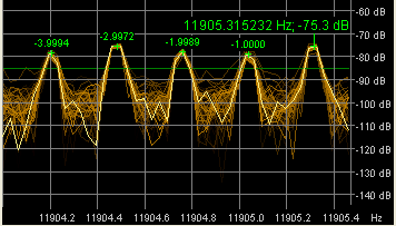
The main peak is marked with the measured frequency (under the assumption that the soundcard still runs at the initial sampling rate), all weaker peaks which obviously belong to the reference signal are marked with relative frequencies as multiples of the nominal periodicity ('spacing' in frequency). For example, '-3.9994' shown in the graphics means 'this peak is 3.9994 times 0.2777777 Hz below the strongest peak', etc. Only peaks which are spaced at (almost) integer multiples of the periodicity are involved in further processing. Peaks below the threshold amplitude (*) are discarded, as well as peaks on obviously 'wrong' frequencies, or peaks which are 10 dB weaker than the main peak. If none of the peaks is close enough to the expected reference frequency, the program uses the measured periodicity value (if 'close enough' to 0.277777 Hz) to find out which peak is the right one. Unfortunately, at the moment this requires a very good SNR (signal to noise ratio) ... so it's more or less a wild guess at the moment ... but this may be improved by 'intelligent averaging' in a future release of the software.
(*) the threshold amplitude, in dBfs, is indicated as a green horizontal line in the scope display
GPS receivers with one-pulse-per-second output (1 PPS output, aka time sync output)
Principle and required hardware for GPS synchronisation
Besides GPS disciplined frequency standards, or even Rubidium or Caesium standards (atomic clocks), some modern GPS receivers are equipped with a PPS output which can be used as a reference signal. Beware, some models are accurate but not precise, others may be precise but not accurate. The author of SpecLab even encountered one unit (btw, not a Garmin) which appeared to be precise (almost no jitter when observing the PPS output on a fast digital storage oscilloscope) but turned out to be not accurate at all - in fact, the PPS output was present on that particular receiver even when no GPS reception was possible - the accuracy was only up to a cheap computer-grade crystal oscillator.
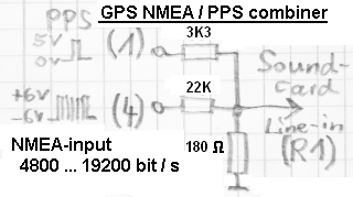
A Garmin GPS 18x LVC(!) receiver gave good results, when used in combination with an E-MU 0202 audio device running at 192 kSamples/second, using the ASIO driver. Most of the GPS-related measurements shown in this document were made with this 'passive' combiner / voltage divider for the PPS- and the NMEA-signal :
If the NMEA output, or the PPS/NMEA combiner shown above is not available, the program can optionally use the PC's system time instead of date and time decoded from the NMEA output. In that case, only the PPS signal (sync pulse) needs to be routed from the GPS receiver into the soundcard, using a simple voltage divider. But this only works if the system time is sufficiently accurate, with a difference between system time and UTC well below 500 milliseconds. More about the two different GPS-sync modes (with or without NMEA) in a later chapter.
- Recommended signal levels :
-
PPS signal (synchronisation pulse) : signal amplitude between 40 and 90 %
of the soundcard's clipping level ("full scale").
NMEA data (serial output, optional, 4800, 9600, or 19200 bit/sec) : signal amplitude between 25 and 50 % of the PPS signal (!) .
The simple voltage divider shown above turns the 5 Volt swing of the PPS signal into 270 mV (peak) for the soundcard,
and the serial output (+/-6 V, RS-232 compatible) into 100 mV (peak) for the soundcard.
For receivers with a TTL level output for the serial data, modify resistor accordingly (10 kOhm instead of 22 k).
See details, and a sample waveform, further below.
- Note:
-
Keep the leads between the GPS output (especially the PPS signal), the voltage
divider, and the input to the soundcard as short as possible. The PPS rise
time must be as short as possible - ideally in the range of a few ten
nanoseconds, even if the soundcard's sampling interval may be as large as
5 microseconds ! Without a 'steep' rise, the pulse location cannot be located
accurately by the software. You can tell that by the waveform of the
interpolated pulse.
The PPS signal must be routed to the soundcard 'line' input, using a voltage divider close to the soundcard's analog 'line' input to avoid overloading it. It may be possible to feed the GPS receiver's serial NMEA data stream into the same soundcard. This allows to retrieve also the calendar date and time from the GPS receiver, not just the time sync pulse (beware, an ancient GPS receiver -not a Garmin- only emitted the UTC time, but not the date). To use the same input line for both PPS + serial NMEA data, both signals must not 'overlap' in time, see sample oscillogram below. The Garmin GPS 18x LVC(!) fulfils this requirement, after setting the baudrate for the NMEA output to 19200 bits per second. This can be achieved with Garmin's 'Sensor Configuration Software', SNSRCFG_320.exe or later. Lower bitrates like 9600 bits/second are be possible if you can manage to turn off all 'unnecessary' NMEA sentences like $GPRMC, $GPGSV, etc. With the GPS 18x LVC configured for GPRMC + GPGGA only (which is sufficient for this purpose), 9k6 serial ouput was ok, and was error-free decodable with a soundcard running at 32000 samples/second (to reduce CPU load for a timestamped VLF 'live' stream).
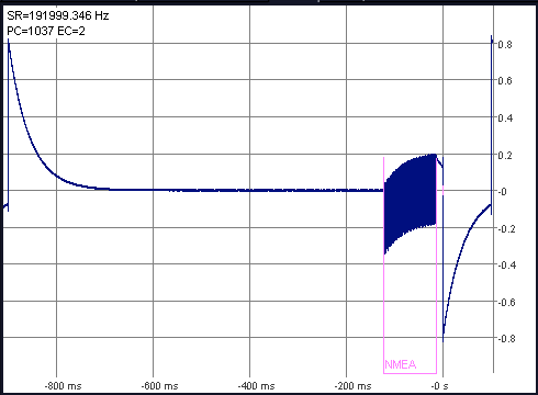
If a combined PPS+NMEA signal shall be used, the amplitude of the PPS signal must be at least two times larger than the NMEA signal - see the example below, from the GPS 18x LVC, with NMEA output at 19200 bits/second. The 'single large pulse' on the left is the PPS signal, the 'data burst' in the center are the NMEA sentences, emitted each second. Note the absence of overlap between the sync pulse (PPS signal) and NMEA data burst, and the significantly lower amplitude of the NMEA signal, which is essential for the software to work properly:
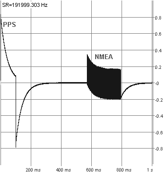
NMEA data from a Garmin GPS 18 LVC via line-input of an E-MU 0202 (left) and Jupiter GPS via notebook's microphone input (closeup, right)
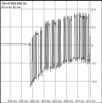
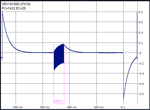
With certain receivers (or receiver configurations), the NMEA data burst may be critically close to the 1-second pulse. Here are two examples from a Garmin GPS 18 LVC, the 1st with a 'less ideal' configuration (more on that in another document) :
- Note:
- It's impossible to feed the PPS signal through a serial port into the program. It must be fed into the same soundcard (or similar A/D conversion device) which also digitizes the analysed analog signal, because otherwise there would be an unpredictable latency between the clock reference and the analysed signal.
If the CPU power permits, run the soundcard at the largest supported sampling
rate (SR). For example, a soundcard which truly supports 192 kSamples/seconds
(*) delivers one
sample point every 5.2 microseconds. But with some DSP tricks, the software
is able to locate the position of the digitized PPS signal up to a resolution
(not a precision) of a few dozen nanoseconds. Only this allows measuring
the SR to fractions of a Hertz once every second .
- Example: If the PPS signal was 'off' by 5.2 microseconds (= one audio sample time) between two pulses, the measured SR would be off by one Hertz (!) :
- 192000 Hz * ( 1 + 5.2*10^-6 ) = 192001 Hz . See notes on the standard deviation of the measured SR at the end of the next chapter.
----
(*) Beware, some crappy audio cards claim to support 192 kS/s, but remove all signals above 24 kHz. It doesn't make much sense to run them at sampling rates above 48 kS/s !
----
How to use a GPS receiver with PPS output to synchronize the soundcard's sampling rate
- Select 'Components' .. 'Sampling rate detector' in SL's main menu.
-
On the 'Sampling Rate Detector' tab, open the 'Reference freq.' combo, and
pick '1 Hz (GPS 1pps)'.
The program will automatically adjust a few other settings then, most notably:
The field 'Mode / algorithm' will be set to 'GPS sync w/ NMEA decoder' . - Select the source channel. This usually 'R1' (= the right input channel from the soundcard); because the left channel ('L1') is already occupied by the analog source.
-
(A) If you built the PPS+NMEA combiner, and want to let the program decode the
NMEA stream via soundcard, enter your receiver's serial bitrate ("baudrate")
for the NMEA output. This is usually 9600 bit/second if you can turn off
all 'unnecessary' NMEA telegrams (possible with the
Garmin GPS 18 LVC). 4800
is usually too slow, because in that case, the NMEA signal would overlap
with the PPS signal as mentioned in the previous chapter.
Make sure that 'Mode / algorithm' is set to GPS sync with NMEA decoder'.
or
(B) Without the PPS+NMEA combiner, only the GPS sync pulse ("PPS") can be fed into the soundcard. For this mode, set
'Mode / algorithm' on the Sampling Rate Detector panel to GPS sync without NMEA.
Caution: Method B is only possible if the PC's system time is accurately set (difference between the PC's system time and the GPS second way below 500 milliseconds) !
The difference between the PC's system time and (minus) the GPS timestamp can be examined as described here. - Set the 'Enabled' checkmark if not already done. Uncheck the 'Measure Only' option (otherwise the soundcard's sampling rate will be measured and displayed, but not taken into account by the rest of Spectrum Lab's components).
-
Switch to the 'Scope' tab (within the calibration
control window) and make sure the PPS pulse is visible there. See chapter
'Checking the GPS PPS signal'.
The PPS signal amplitude must exceed 10 % of the audio input's clipping level, but shouldn't exceed 80 % of the clipping level.
The NMEA signal amplitude must not exceed half the amplitude of the PPS signal, but shouldn't be less than 10 % of the clipping level. See details in the previous chapter, titled GPS sync hardware.
After two seconds(!), the SR detector status (indicator near the bottom of the 'Sampling Rate Detector' tab) should turn green, and the sample rate deviation gets dumped into the 'History' window (numeric value in ppm). The proper function of the GPS receiver, and the SR detector can be monitored on the same tab. Example:
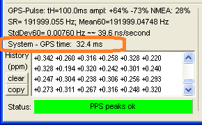
The parameters shown on the SR Detector tab are (..subject to change..) :
| GPS-Pulse : tH = <logic-high pulse duration of the sync pulse, typically
100 ms> ampl = < positive and negative peak amplitude, relative to full scale> SR= < current measured sample rate, from last second> Mean60=<mean / average over 60 seconds> StdDev60= < standard deviation of the measured sampling rate, from last 60 seconds> also scaled into 'nanoseconds per second' = ppb (parts per billion) |
A standard deviation of approximately 30 nanoseconds per second (one PPS interval) was measured with a Garmin GPS 18x VLC, connected to an E-MU 0202 running at 192 kSamples/second for a few hours in a thermally 'stable' environment. Don't be fooled by this, it's not the accuracy of the system, since the GPS 18x datasheet specifies an accuracy of the PPS output of +/- 1 microsecond at rising edge of the pulse. Fortunately, the Garmin's PPS output jitter was way below 1 us, and the sync pulses from two receivers were less than 40ns apart (with 12 satellites in view).
Note: The EMU-0202 and a few other cards inverted the pulse polarity ! The software automatically corrects this, by examining the PPS signal's duty cycle: If the time between rising and falling edge of the PPS signal exceeds half the cycle time (i.e. 0.5 seconds in most cases), the signal is inverted. Thus the 'interpolated PPS signal', displayed on the SR calibrator's scope tab as explained in the next chapter, always shows the 'important' rising edge.
Checking the GPS PPS signal
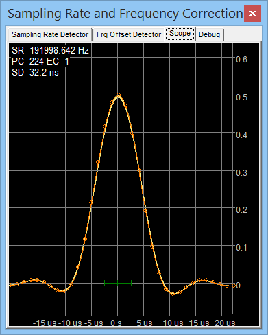
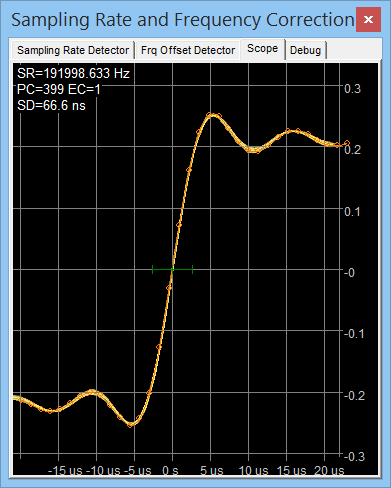
The waveform of the interpolated GPS pulse can be observed on the calibrator's scope panel. A 'good' pulse rises within a few microseconds (limited by the soundcard), as in the following screenshot on the right. Some GPSes emit very short pulses (e.g. Trimble Thunderbolt E : 10 us), which should look as shown on the left screenshot below. The standard deviation in the recent 60 sync pulses is also shown here ("SD"), because it's a good quality- and jitter indicator.
The green horizontal line in the center marks one sample interval (here:
1 / 192kHz = approx. 5.2 µs ). The yellow curves show subsequent pulses
(option 'slow fade image' in the context menu);
they should ideally coincide. If they don't (but turn into a broad blurred mess),
there's a problem with jitter, noise, hum, or a bad soundcard.
The orange curve shows the most recent pulse, small circles are the interpolated points
(can also be activated through the context menu, i.e. mouse click into the
curve area). As in some other scope modes, you can zoom into the graph by
pulling up a rectangular marker - see next chapter.
Again: You don't need to have the NMEA output if the GPS receiver shall 'only'
be used to improve the accuracy of the soundcard's sampling rate. But with
a GPS receiver with a PPS- and a serial NMEA-output, the latter
can be decoded through the soundcard (and you will have a reliable
time source for free, even when not connected to the internet). First check the
recommended signal levels on
the scope, as explained above. If the combined waveform (PPS plus
NMEA) looks ok, open the GPS (NMEA) Decoder
Window through SL's main menu, or click on the 'Show GPS' button in the
Sample Rate Detector control panel.
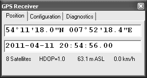
The position (latitude, longitude, and height above sea level) is displayed
on the 'Position' tab. The
display format can be changed on the decoder's
'Configuration' panel. The 'raw'
NMEA sentences can be examined on the
'Diagnostics' panel.
Notes:
Waveform of the interpolated pulses of the PPS signal.
Multiple pulses are superimposed to check for noise / jitter.
Left: Very short pulse, or differentiated pulse edge for centroid calculation.
Right: Rising edge of a 'long' pulse, not differentiated, used by old algorithm.
Checking the GPS NMEA signal (and
decoding it via soundcard)
Don't trust the presence of a sync pulse (pps) alone - see notes at the begin
of this chapter.
An 'automatic' detection didn't work reliable (in 2015), thus the option
'GPS 1 second late' was added as a checkmark on the Sampling Rate Detector tab.
The next chapter describes how to test if this option has been properly set.
Checking the GPS NMEA timing (is it "one second late" ?)
In 2015-01, a problem was noticed with the timing between a GPS receiver's NMEA- and Sync Pulse output
(see previous chapter).
To defeat the problem described there, the new option 'GPS one second late' was added
on the Sampling Rate Detector tab.
Screenshot of a part of the 'Sampling Rate Detector' panel in SL.
Note the checkmark 'GPS 1 second late' in the lower right corner.
To test if the GPS (NMEA-) based timestamps are ok, a second (well-known) time signal is required. Here, for example, DCF77 (the German time signal transmitter on 77.5 kHz) on a fast-running spectrogram with correct timestamps. The signal can be picked up in Europe with a piece of wire connected to the input of a soundcard with 192 kSamples/second. The missing amplitude gap in the 59th second of each minute confirms that the option 'GPS 1s late' has been properly set (or, in this case, cleared).

Fast running DCF77 spectrogram with missing amplitude gap in the 59th second of the minute.
The pseudo-random noise is interrupted each second, but the carrier is not reduced.
If the difference between 'System time' minus 'GPS time' is well below 500 milliseconds,
the current setting of the 'GPS one second late' option is ok.
The 'Scope' tab (in the sample rate calibrator's control window)
Left side: Coherent reference signal (10 kHz), Goertzel filters running, graph on the 'Scope' window shows the narrow-band spectrum around the reference signal. The last result of the frequency measurement, and the magnitude of the reference signal are shown near the peak in the graph.
Right side: One pulse-per-second signal from a GPS receiver, graph showing the interpolated rising edge of the sync signal.
Other display modes can be selected on the "Sampling Rate Detector" tab, and a few options can be modified through the scope's context menu. Click into the graph area, or drag a rectangular marker to zoom in / out.
By default, the old graphs (from previous spectrograms) slowly fade out on the display. This is not a bug but a feature ;-) ... it helps to discover intermittent noise, dropouts, or "slowly drifting" signals without the need for a spectrogram display. The most recent curve is yellow; older curves fade to brown, and finally disappear after a couple of minutes. Peaks which look 'smeared' on the display are not stable in amplitude or frequency (or, for the GPS sync pulse, suffer from jitter). The 'slow fade' option can be turned off through the context menu, too.
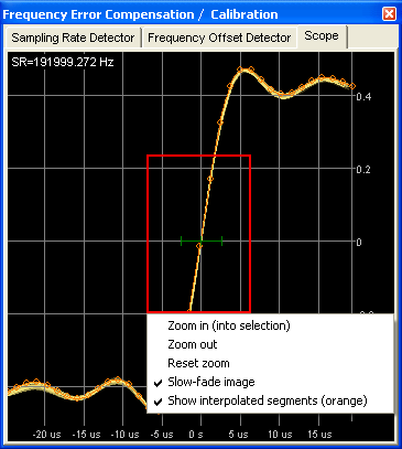
To zoom into the graph, move the mouse pointer into the upper left corner of the 'region of interest', press and hold the left button, while moving to the lower right corner. Then release the mouse, and select 'Zoom in' in the menu. 'Zoom out' zooms out by about 50 percent. 'Reset zoom' zooms out completely.
See also: Scope display in GPS / PPS mode ; Spectrum Lab's more advanced time domain scope ; Details on connecting GPS receivers .
The 'Debug' tab
The 'Debug' tab in the frequency- and sample rate calibrator window is only used
for troubleshooting and software tests.
During normal operation (with a 'good' input signal), the message list should
remain almost empty. Whenever the sample rate calibrator (or frequency calibrator)
encounters a problem, it will append an error message (unless the error display
is paused). Most of the error messages and warnings should speak for themselves,
thus only a few of the possible messages are listed below.
- PulseDet: Excessive SR drift (-0.400 Hz²)
The sample rate drifts faster than expected (more than +/- 0.025 Hz per second).
If this warning only occurs once, it's just a subsequent error of 'noise' that can be ignored.
Interpreter commands for the frequency calibrators
fo_cal.xxxx = commands and functions for the frequency offset calibrator:
-
fo_cal.avrg
Average frequency offset (difference between "measured" frequency and "known reference" frequency ).
A positive offset means "the measured frequency is TOO HIGH". So to correct a "measured" frequency, subtract fo_cal.avrg from the measured value before you display it (but beware: Do NOT subtract fo_cal.avrg if the FFT frequency bins have already been corrected as explained here ). -
fo_cal.delta_phi
Phase angle difference between to consecutive phase calculations. Should ideally be zero. Mainly used for program development. -
fo_cal.fc
Current center frequency which has been measured by the frequency offset calibrator. Should ideally be the same value as the "known reference frequency". You may (ab-)use this function for a precise measurement of a single frequency. Example: To measure the exact mains frequency ("hum"), set the "Reference audio frequency" to 50.000 Hz, the "observed bandwidth" to 0.5 Hz, and the max. offset also to 0.5 Hz (all these values on the control panel of the Frequency Offset Detector).
sr_cal.xxxx = commands and functions for the sampling rate calibrator:
-
sr_cal.sr
Momentary, non-averaged, measured sampling rate. -
sr_cal.avrg
Averaged measured sampling rate. This value is also displayed in the calibrator's control window. You may use it for your own application. -
sr_cal.ampl
Measured amplitude of the reference signal, converted into dBfs (decibel over full scale, thus always a negative value). -
sr_cal.delta_phi
Phase angle difference between to consecutive calculations. Should ideally be zero. Mainly used for program development. -
sr_cal.fc
Measured reference signal frequency. Calculated by the sampling rate calibrator, under the assumption that the sampling rate was constant since the calibrator was started. Should ideally be the same value as the "known reference frequency". Useful for plotting the audio device's oscillator drift, if a drift-free frequency reference (OCXO, GPS) is available. -
sr_cal.fr
Returns the configured reference frequency (nominal frequency, constant), as configured in the 'Reference Frequency' field . - sr_cal.systimediff
Returns the difference, in seconds, between the PC's system time and the time decoded by the sampling rate calibrator (for example, from the GPS/NMEA decoder). The same value is displayed as 'System time minus GPS time' on the SR calibrator control panel.
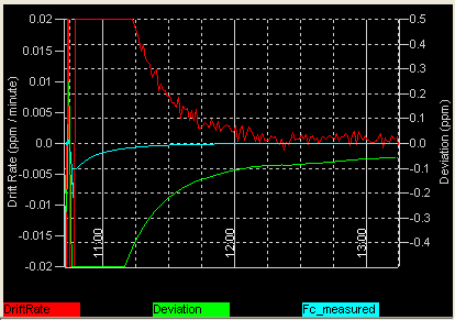
See also: Example for plotting the soundcard's frequency deviation (in ppm) and the drift rate (in ppm / minute), Interpreter command overview, circuit window, main index .
See also: Spectrum Lab's main index .
Appendix
Soundcard clock drift measurements
The following drift rate (red graph in the diagram below) and frequency offset (green) graphs were made with an internal audio device in a notebook PC (Thinkpad Z61m, internal "SoundMax HD Audio"). The graph starts a few minutes after booting the PC. Before that, the PC had cooled off for several hours. The reference signal (10 MHz OCXO divided down to 10 kHz) had been running for a couple of days. The soundcard's final sampling rate was calibrated earlier (in the calibration table).
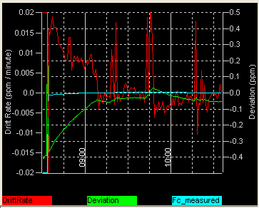
Sampling rate drift test (Thinkpad, internal audio device)
Each horizontal division is 15 minutes wide. At 09:10, the notebook's cooling fan started to run, causing the 'bent' curve. The green graph shows the deviation of the sampling rate; vertical scale range for this channel is +/- 0.5 ppm (parts per million - see formula at the end of this chapter). The same order of clock deviation can be expected when measuring frequencies without the continuous sampling rate calibrator.
Next test candidate: An E-MU 0202 USB (external audio device in a quite large box). The initial sampling rate deviated from the final value by over 2 ppm, so during the 'early' warm-up phase, the trend is only visible on a broader scale (in cyan colour). 5 minutes after start, the calibrator's tracking algorithm was able to measure and eliminate the drift (because of the large initial drift rate, and the 30-second frequency measuring intervals for the Goertzel filters). It's obvious that the curves are less 'jumpy' than with the internal soundcard, thanks to the absence of a cooling fan in the box.
Sampling rate drift test (E-MU 0202, USB audio device)
To measure and plot the soundcard
oscillator's drift, the interpreter function
"sr_cal.fc" were used, and SL's
plot window . The expression
1E6*(sr_cal.fc-sr_cal.fr)/sr_cal.fr calculates the current frequency
deviation in ppm (parts per million).
To measure the drift rate (in ppm per minute), calculate the drift
(frequency error in ppm) periodically, and subtract the previous result from
the current result every minute. This can be achieved in the
Conditional Actions table ("DriftRate
= Drift - OldDrift", which is not true maths but it works for this purpose).
The 60 second timebase is provided by one of SL's programmable
timers. Example (copied from the
conditional actions in the configuration 'SoundcardDriftTest.usr') :
| Nr | IF.. (event) | THEN.. (action) |
| 1 | initialising | Drift=0 : DriftRate=0 : OldDrift=0 : timer0.start(60) : REM timer will run off after 60 seconds |
| 2 | timer0.expired | Drift=1E6*(sr_cal.fc-sr_cal.fr)/sr_cal.fr : DriftRate=Drift-OldDrift : OldDrift=Drift : timer0.start(60) |
The values of 'Drift' (in ppm) and 'DriftRate' (in ppm / minute) are plotted in the watch window. The sample application (SoundcardDriftTest.usr) is contained in the SL installer.
Sample Rate Calibration Algorithm
(Old algorithm, Rev date 2002-04-18, only uses one complex oscillator, one complex multiplier, and a long chain of decimators):
The example explained here uses a reference frequency f_ref = 15625 Hz (TV line sync)
-
NCO frequency for the I/Q mixer
theoretically: f_ref = 15625 Hz (this is the 'Reference Frequency' entered by the user)
practically : f_nco = f_ref * k, where k = true sample rate / assumed sample rate,
because the program only THINKS it mixes the input signal with f_ref, but in fact -due to the sample rate error- the true NCO frequency is different !
Here for example: k = f_sample_assumed / f_sample_true = 44101 Hz / 44100 Hz,
so f_nco = 15625 Hz * 44101/44100 = 15625.35431 Hz. The NCO is initially programmed for '15625.0 Hz' because the program does not know the true sample rate (this is what we're looking for !) -
Frequency at the output of the I/Q mixer (not decimated)
f_mix = (f_ref - f_nco) = f_ref - f_ref*k = f_ref * (1-k) = 15625 Hz * (1-44101 / 44100) = -0.3543 Hz
(dont bother about the negative frequency, we are processing I/Q samples) -
Accumulation of the phase (from f_mix_decimated, observed over the measuring
interval)
Measuring interval: t_meas = decimation_ratio / true sample rate = 16384 / 44101 Hz
Phase deviation: delta_phi = 360° * t_meas * f_mix = -47.3866°
(the phase deviation is what the software actually measures. It does not know the true sample rate !) -
Calculation of the 'calibrated' sample rate.
known: delta_phi, f_ref, decimation_ratio, f_sample_assumed
wanted: k (correction factor), f_sample_true
delta_phi = 360° * t_meas * f_mix
= 360° * (decimation_ratio * f_mix) / f_sample_true
= 360° * decimation_ratio * (f_ref - f_ref * f_sample_true / f_sample_assumed) / f_sample_true
-> ... ->
f_sample_true = f_sample_assumed / ( 1 + delta_phi * f_sample_assumed / (360° * decimation_ratio * f_ref) )
Note that the NCO frequency is not reprogrammed with the new "true value" of f_ref !
(New algorithm, Rev date 2010-03-30, uses a bank of Goertzel filters to calculate a DFT for a few frequencies):
< ToDo >: Describe how the phase information in the complex DFT can be used to measure the frequency with a resolution of a few microhertz, using a 30 second measuring interval...
MSK Carrier Phase Detection
To detect the 'carrier phase' of an MSK signal (without demodulating or decoding it), the complex, downconverted (analytic or "baseband") signal is squared. This produces two discrete lines in the spectrum, symmetrically around the carrier frequency.
For example, DHO38 is first multiplied with an complex NCO (numerically controlled oscillator, with sine- and cosine output) at 23400 Hz, then decimated until the sampling rate is about 1.5 to 3 times the bitrate. In the decimated, complex (analytic) signal, the two lines appear like 'sidebands', separated -100 Hz and +100 Hz from the carrier signal (which is now at 0 Hz, ideally).
The squared baseband signal is then passed through a DFT (discrete fourier transform, possibly an FFT = Fast Fourier Transform). To avoid locking on false signals, the amplitudes in the complex frequency bins (at the two "expected" baseband frequencies) are compared with their neighbours, and the phases in the complex bins are compared with the previous DFT (in reality, this step is a bit more complicated because the signals are not perfectly centered in their FFT bins.. some phase angle fiddling is required for this reason).
Compared to a continuous wave signal, the MSK carrier phase detection requires a larger SNR (go figure..) because the observed signal bandwidth (or, the equivalent receiver bandwidth) is larger. For comparison, measuring the carrier phase of DHO38 requires approximately a 300 (!) Hz filter bandwidth. For phase coherent time signal transmitters like DCF77, the observed bandwidth may be less than 1 Hz.
Note: The same principle is also used in the phase- and amplitude monitors (when configured for MSK).
Last modified : 2021-05-16 (now using CSS for chapter / headline numbering)
Benötigen Sie eine deutsche Übersetzung ? Vielleicht hilft dieser Übersetzer - auch wenn das Resultat z.T. recht "drollig" ausfällt !
Avez-vous besoin d'une traduction en français ? Peut-être que ce traducteur vous aidera !