Time-domain scope
Contents
- Introduction
- Controls on the left side of the window
- Zooming and scrolling the display
- Oscilloscope mode
- Trigger modes
- 'Specials' (tab)
- Settings (on various tabsheets)
- Presets
- Interpreter commands and -functions for the time-domain scope
- Appendix
- Loran GRI table (for precise-sync trigger)
See also: SpecLab's main index , Component window , sample rate calibration .
Time domain scope - Introduction
Besides the analysis of signals in the frequency domain, you can use Spectrum Lab for an analysis of waveforms in the time domain. It works, to some extent, like a digital storage oscilloscope - but with a very limited bandwidth.

To open the time-domain scope in SpecLab, select "View/Windows"..."Time Domain Scope" in SL's main menu, or click on the Time Domain Scope box in Spectrum Lab's circuit window. Please note that even if the time domain scope's window is visible, the scope function itself may be turned off to save CPU power (especially on slower machines you will see that the scope is a big eater of calculation power). You can turn the scope function on and off through the scope's "Mode" menu.
One or two input channels may (or must, depending on the mode) be connected to the scope. You can select the sources in the combo boxes on the left side of the scope screen, but it's easier to select the inputs in the circuit window, where you can also see all available sources. Other controls on the left side of the scope window are explained in the next chapter.
Note: If any of the inputs is connected to a "currently unavailable" source, the scope display may pause (for example, if one of the scope's inputs is connected to the right input channel of the soundcard, with the card not running in stereo mode). Usually, only available sources are listed in the combo box, but if you change the audio settings afterwards these sources may become unavailable.
The scope can be triggered either with its built-in trigger (which is quite simple) or with the external "Universal Trigger Block" (part of the test circuit, offers more flexibility). The universal trigger can be used to trigger the scope and the spectrum analyzer simultaneously, which is impossible with the scope's built-in trigger.
All scope settings can be saved as part of a Spectrum Lab configuration file (*.ini or *.usr), so you can quickly switch from one configuration to another through SL's Quick Settings menu. For many common applications, there is a set of preconfigured settings (scope settings only) in the scope's menu ("Presets"). There is ...
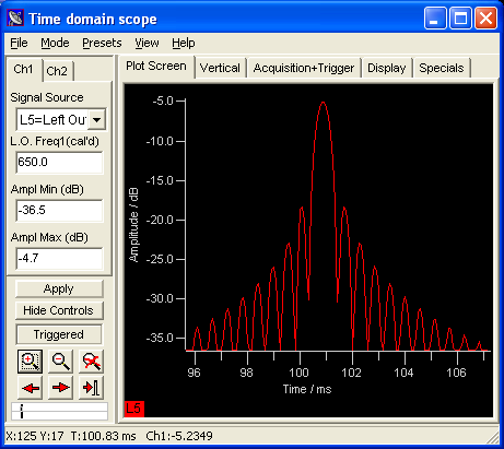
- an oscilloscope with one or two channels (see screenshot above)
- several frequency-selective phase meters
- a very special application called "Loran monitor"
- and another preconfigured setup called "Lissajous figure", which is in fact the X/Y scope mode without trigger, used for phase/frequency comparations in the old days of analog oscilloscopes. Use it for nostalgic reasons or educational purposes - remember the lissajous figure of two signals of same amplitude, same frequency but 90° phase difference ? Some radio amateurs use similar displays to tune the mark/space-filters in their RTTY decoder.
Controls on the left side of the scope window
The following controls (buttons etc) are located in a resizeable area on the left side of the scope window:
-
 Zoom in (into the
current selection, marked with the mouse; or if there's no selection, by
a factor of two until the maximum is reached)
Zoom in (into the
current selection, marked with the mouse; or if there's no selection, by
a factor of two until the maximum is reached)
-
 Zoom out
-
 Reset zoom (so that one pixel along the X
axis represents one sample again)
Reset zoom (so that one pixel along the X
axis represents one sample again)
-
 Scroll left
-
 Scroll right
-
 Scroll towards the trigger position
-
-
 Horizontal
'scroll' indicator.
Horizontal
'scroll' indicator.
-
The inner (black) rectangle represents the currently visible area. You can
pull this frame with the mouse to pan horizontally.
The outer (gray) rectangle represents the display buffer. The size of that buffer (number of samples) can be adjusted in the settings.
When operating in one of the triggered modes, a small 'pulse' marks the theoretic trigger point, depending on the pretrigger setting.
Fine horizontal scrolling is also possible by grabbing the time scale with the left mouse button, at least in Y(t) 'Oscilloscope' mode.
Most of the buttons are grayed if a function is not available (for example, if the maximum magnification is already reached, the "zoom in" button will be disabled).
Zooming and scrolling the display
Depending on the current zoom setting and the size of the display buffer, the scope display can be scrolled horizontally (along the time scale) and vertically (along the amplitude scale). There are no extra scroll bars for this; just grab and move the scale with the left mouse button (starting outside the curve area; because otherwise you would open a marker frame to zoom into).
For the vertial scale ("Y" axis), you can modify the upper end, lower end, or both ends of the displayed amplitude range:
-
grab the scale in the upper quarter (i.e. press and hold the left mouse button above the upper end) to modify only the upper end ("Ampl Max");
-
grab the scale in the middle part to modify both ends ("Ampl Min" and "Ampl Max"), i.e. scrolls the display vertically without zooming in or out;
-
grab the scale in the lower quarter to modify only the lower end ("Ampl. Min").
You can also modify the amplitude range numerically by modifying the fields "Ampl Min" and "Ampl Max" on the tabsheets "Ch1" or "Ch2" at the left side of the scope window.
Fast scrolling is possible with the scroll buttons.
Oscilloscope mode
In "oscilloscope" mode, a signal can be plotted as a function of time. It's possible to
-
display one or two channels with common or individual vertical scaling
-
use one of different trigger modes
-
reduce the bandwidth of the input (by decimation)
-
display peaks and/or average value, depending on the timebase settings
Like most oscilloscopes, this one can also be switched into X/Y mode. In
this mode, both channels must be active (turned on in the "Mode" menu). The
first channel is used for X-deflection, the second for Y-deflection. The
trigger is pretty useless in X/Y mode, even though it works. An
important parameter for X/Y mode is the persistance, which can be set on
the "Display" tab under "Miscellaneous". A persistance of zero means
eternal persistance, which means pixels will not disappear
once they are plotted !
Trigger modes
There is a simple trigger function, mainly intended to be used in Y(t) mode ("oscilloscope") but you can use the trigger also in other modes. The trigger settings can be defined on the scope's "Acquisition + Trigger" tab, where you will find these options - or maybe more:
Trigger Mode : Select one of the following:
-
OFF (untriggered roll)
-
AUTO: If a trigger signal is detected with the current 'level' setting, the display is triggered, otherwise the display will be updated without a trigger. This is also the default mode for many analog oscilloscopes, because "you always see something even with the wrong trigger settings".
-
NORMAL: The display will only be updated if there is a trigger event. Without a trigger signal, the display will freeze (usually due to a wrong setting of the trigger level). As with analog oscilloscopes, the AUTO mode is more frequently used than the NORMAL mode.
-
SINGLE SHOT: The trigger only fires once, then the display will freeze until you start it again (manually).
Slope: Allows you to select
-
Rising or
-
Falling edge of the trigger signal.
Source: Defines the source of the trigger signal..
-
Sync Interval Generator (internal)
-
Channel 1 (internal)
-
Channel 2 (internal)
-
External Trigger: If this option is selected, the "Universal Trigger Block" (part of the test circuit) replaces the scope's internal trigger. In this mode, all other controls in the "Trigger" control panel have no function - including the trigger mode, slope, coupling, etc because the Universal Trigger has its own control panel (a popup menu in the circuit window).
Trigger coupling: Select
-
"DC" for direct current, or better
-
"AC" for alternating current here, because some soundcards have a quite large offset error, which means the permanent level is not zero if there is no input signal !
Pretrigger: Most analog oscilloscopes start the scan in the moment when the trigger fires, so the trigger event can often not be displayed completely. This is the case when the pretrigger is set to 0 % (percent). With 50 percent, the trigger event will be visible in the middle of the scope area. With 100 percent pretrigger, you will only see the PRE-TRIGGER history (pre = "before"), and the trigger event would be at the right edge of the screen. The amount of pre- and post-trigger samples is also indicated in the horizontal position indicator on the left control panel.
Level: The trigger will fire when the input signal crosses this level (~voltage). The trigger level is entered as a 'percentage of full scale', but with both possible signs, i.e. a meaningful range is -100 to +100 % . With the trigger level set to 0 (%), and the trigger source is set to 'Channel 1 (internal)' or 'Channel 2 (internal)', a trigger occurrs on a rising or falling slope, when the input voltage just crosses zero.
tSync: Interval time of the sync generator in seconds. Only has an
effect if the trigger source is set to "Sync Interval Generator". This can
be used if to observe periodic signals with well-known frequency, for example
the 50 (60) Hz mains, etc. Below the edit field, the reciprocal of the interval
time (= the frequency) is displayed. Remember that -like in many other input
fields of SL- you can not only enter a fixed numerical value but also an
expression ("formula"). So, for example, if you want to set the sync interval
generator to 60 Hertz, enter "1/60" in the field and hit the Enter/Return
key to apply the edit. After evaluation, the calculated result will be visible
in the edit field.
The sync generator was a nice tool to play with when hunting for worldwide
Loran stations as explained here.
Triggered Average
In triggered Y(t) mode, a special mode is available where each horizontal
position on the screen (more precisely: each index in the display buffer)
has its own moving average filter. The oscilloscope screen will then show
the average of the last 4, 16, 64, 128 .... 32768 horizontal scans. This
feature can be used to make weak periodic signals visible in the time domain,
for example short pulses which would otherwise (without the averaging) get
lost in the noise.
One example which uses this function is the Loran
Monitor described further below. The number of averages (per sample point)
can be modified on the 'Acquisition +
Trigger' tab.
'Specials' (tab)
The scope's 'Special' tab once contained a few rarely used features. Most of them have been removed or replaced by other function blocks.Phase meters
The phase meters have been removed from the time scope. A better, and more
versatile replacement is the pam() function
(phase- and amplitude monitor),
which is intended to be used in SL's watch / plot
window.
Settings (for the time domain scope)
Due to a lack of space in the scope's window, the settings are organized on various tabsheets (not really logical...). Most of the settings should be self-explanatory; so here just a few:
Vertical
The setting on the 'Vertical' tab affect the vertical axises of the displayed channels.
Note: The vertical display range can be set in the 'controls on the left side' of the scope
window, which can be visible along with the 'Plot Screen' tab.
The controls on the 'Vertical' tab include:
- Logarithmic or linear scale, plus the reference value for 0 dB (usually 100 % = full input swing of the A/D converter)
- Display style (lines or single pixels for each sample)
- Turn a channel on and off (for the display).
Note: The first channel can not be turned off. - 'Show Controls' (button):
Switches to another tabsheet on the left side of the scope window, where the vertical scaling for this channel can be adjusted ('Ampl. Max', 'Ampl. Min', both measured in 'percent of full scale', i.e. -100 % .. +100 %)
Acquisition and Trigger
Defines how, and when new samples are acquired. Decimation means reduction of the input sampling rate. For example, if the oscilloscope is connected to a signal with 96 kHz sampling rate, but you are only interested in low-frequency signals, you can decimate the sampling rate by the next suitable power of two to reduce the bandwidth (and the CPU usage caused by the scope). Also, reducing the sampling rate this way gives a longer "timebase" (which could be achieved with a larger sample buffer, and zooming out, at the expense of a higher CPU usage).
The 'Trigger' modes should sound familiar, if you ever used a hardware oscilloscope. If not ...
- "Auto" means the oscilloscope will start to measure, if there is no trigger signal ("no input").
- For most analog scopes, this is the default mode because you always 'see something' on the screen.
- "Normal" trigger means, the oscilloscope will only capture new samples if a trigger event has been detected.
- If there is no trigger (because, for example, the trigger level was not reached), the scope will show nothing (not even a flat line).
The 'Averages' field defines the number of averages displayed on the screen, which can be used to reduce to dig weak periodic signals (especially pulses) out of the noise. More details here. Note that this kind of averaging only makes sense in triggered modes. Each sample in the display buffer has its own moving-average filter. The amount of memory required for this function can be quite large, especially with a large display buffer (see below), and a large number of averages.
Display
Controls on this tabsheet of the time domain scope:
- display buffer size: Number of samples captured in the oscilloscope's sample buffer (for each trigger event). When set to zero, the scope only captures as many samples as it can display on the screen. Using a large number allows you to 'pan around' and zoom in/out later, using the controls on the left side of the scope window.
- Scale: Horizontal magnification (applied when drawing the graph). 100 % means one sample will be mapped to one horizontal position ("pixel coordinate along the X axis"). Values below 100 % mean the output will be compressed on the screen ("zoomed out"), values above 100 % mean zooming in. Instead of modifying this parameter numerically, use the zoom buttons .
- Colours: Modify the colours of curves and grids, etc.
Presets
For a quick start, there are a couple of 'preset' configurations for the time domain scope.
Here just some of the presets, there may already be more:
Two Channel Oscilloscope
This is a simple dual-channel oscilloscope. Per default, channel 1 is coupled to the left audio input (ADC), Channel 2 to the right channel. Both vertical scales are set for 'maximum range', so a common vertical axis appears. Timebase settings are set for 'no decimation', trigger is enabled, trigger source is channel 1. If no trigger signal is detected for some time, the scan starts automatically ('auto-trigger').Loran Monitor
A special application for longwave listeners. Tune your AM receiver to 100kHz and connect it to the soundcard. Unless the last Loran chain has been demolished in the meantime, there will be a 'rattling' sound originating from a system of navigation aid transmitters with (at least once) worldwide coverage. The preset 'Loran Monitor' is a special Y(t) diagram with the trigger driven by a sync-interval generator, programmed to pick up some of these transmitters. The interval is (by default) set to 0.07499 seconds, which is the Group Repetition Interval (GRI) of the Sylt and Lessay transmitter. The display runs in 'average' mode to reject noise. After a couple of seconds, the Loran pulse train should appear. With an other GRI value (can be found in the appendix), you may be able to dig other Loran stations out of the noise. If required, set the 'average' value higher. If the pulse train slowly moves left or right, the sampling rate of your soundcard is not properly calibrated. The Loran transmitters (if they still exist) are used as navigation aid, their stability is excellent, similar to the more recent GPS system (but Loran is much simpler to receive, and due to the low frequency, the antenna doesn't need a clear sky view).Note: The average value is drawn as a line, while the min+max values are only drawn here as single dots. This avoids a crowded screen, but you can still see the pulses from other Loran transmitters (with different GRI's).
Chirp Radar Display
This special configuration was added 2010-02 in Spectrum Lab for experiments with a bistatic, chirped, backscatter radar for amateur radio use on HF or VHF. It is based on ideas presented by Andrew Martin (VK3OE) on the VK Logger forum . The time domain scope was used as a 'graphic frontend' for the radar receiver.
Lissajous figure
In this mode, channel 1 is used for 'X' deflection, channel 2 for the 'Y' deflection. This can be used for crude phase comparation (circle = 90° phase difference etc), or as a RTTY tuning scope (connect Ch1 to a MARK frequency filter and Ch2 to a SPACE frequency filter, realized either by software or hardware).Note: The 'persistance' value of the display can be adjusted, the optimum value for a good and not too crowded display depends on the signal frequency and the amount of noise.
Interpreter commands and -functions for the time-domain scope
A few parameters and current values inside the time domain scope can be accessed through the interpreter. This can be used (for example) to plot data in the watch/plot window. For example, a long-term phase plot may be exported to a text file for further post-processing.
The following interpreter functions are implemented for the time domain scope (remember: a function returns a value, a command does not):
-
tds.ch[X].ampl
returns the current amplitude from channel X (0=first channel, 1=second channel, indices start at zero !) -
tds.ch[X].phase
returns the current phase from channel X
See also:
back to the overwiev of the time-domain scope
Appendix
Loran table
If you have a longwave receiver for 100kHz (AM or SSB), you can use the preset "Loran Monitor" to watch the pulses on the screen. The following table has the "Group Repetion Intervals" for most Loran stations worldwide.
Note: In February 2010, most of the US American stations (except the Russian-American) were closed down. So it may be a matter of time until this trusty old navigation aid has disappeared completely (in favour of satellite navigation systems like GPS, GLONASS, etc).
Loran Table
| GRI (master) | GRI 2 | GRI3 | Location of transmitter |
| 7499 | 6731 | 9007 | Sylt |
| 6731 | 7499 | Lessay | |
| 7001 | 9007 | Bo | |
| 9007 | 7001 | Eide | |
| 8000 | W Russia | ||
| 7990 | Mediterranean Sea | ||
| 7270 | 5930 | ||
| 5930 | 9960 | 7270 | |
| 5980 | 7950 | 9990 | Russian-American |
| 9990 | 5980 | 7960 | |
| 5990 | 8290 | 7960 | |
| 8930 | 9930 | 7950 | |
| 9940 | 5990 | ||
| 8970 | 9960 | ||
| 7960 | 9990 | ||
| 8290 | 8970 | 9610 | |
| 9960 | 8970 | 5930 | |
| 7980 | 8970 | 9610 | |
| 9610 | 8970 | ||
| 6042 | Bombay | ||
| 5543 | Calcutta | ||
| 7950 | 5980 | Eastern ex USSR | |
| 6780 | 8390 | China South Sea | |
| 7430 | 8390 | China North Sea | |
| 8390 | 7430 | China East Sea | |
| 9930 | 8930 | East Asia | |
| 8830 | 7030 | Saudi Arabia North | |
| 7030 | 8830 | Saudi Arabia South | |
Note: A GRI of 7499 is a group repetition interval of 0.07499 seconds.
This value must be entered in the 'tSync' field on the trigger sheet if you
want to dig such a signal out of the noise with high "average" value..
Last modified : 2020-10-23
Benötigen Sie eine deutsche Übersetzung ? Vielleicht hilft dieser Übersetzer - auch wenn das Resultat z.T. recht "drollig" ausfällt !
Avez-vous besoin d'une traduction en français ? Peut-être que ce traducteur vous aidera !