
Spectrum Lab Circuit Components
Contents- Spectrum Lab circuit components - Introduction
- Signal Processing Circuit and the 'Component' Window
- The 'Component' Window
- Monitor Scopes
- Universal Trigger Block
- Counter / Timer (pulse- or event counter, operating in the time domain)
- Input Preprocessor
- Test Signal Generator
- Programmable Audio Filter
- Frequency Converter ("mixer")
- Audio input and output
- Output- and "cross coupling" amplifiers
- Spectrum analyser
- DSP Black Boxes
- Signal processing sequence (in each DSP Blackbox)
- Adder or multiplier (to combine two input channels in a DSP blackbox)
- Bandpass Filter (in a DSP blackbox)
- Delay line in a DSP blackbox
- Advanced hum filter in a DSP blackbox
- Hard Limiter in a DSP blackbox
- Noise Blanker in a DSP blackbox
- DC Reject / DC measurement (in a DSP blackbox)
- Modulators and Demodulators in a DSP blackbox
- Automatic Gain Control (in the DSP blackboxes)
- Chirp Filter (in the DSP blackboxes)
- Sampling Rate- and Frequency Offset Calibrator
- The 'Component' Window
- Interpreter commands for the test circuit
Spectrum Lab circuit components - Introduction
Spectrum Lab is more than a simple audio spectrum analyser. It can be used for other purposes like filtering, decoding, receiving & demodulating VLF signals with the soundcard (or other audio input devices). Most of the circuit components listed in subsequent chapters of this document can be be activated or controlled in the Component Window.Some circuit components (like the 'Signal Generator') have their own control panel / window, explained in separate documents (e.g. the Signal generator control window).
See also: Spectrum Lab's main index, 'A to Z', sample applications .
Signal Processing Circuit and the 'Component' Window
The 'Component' Window
This window shows an overview of the main function blocks in a "circuit-like"
style. It can be opened from SL's main window (View/Windows...Components).
Note: There may be more components in the component window than shown here.
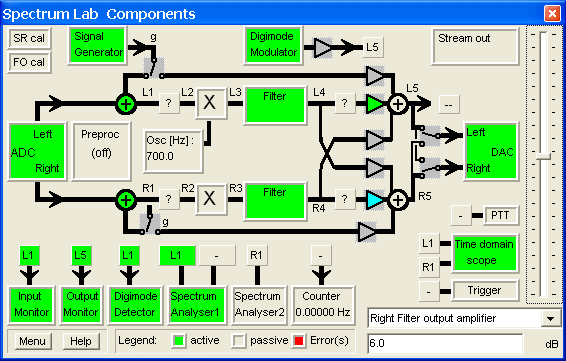
The actual state of most components is indicated by their color. Green means active, gray=passive, red=error(s) occurred; not shown in the legend: light blue means "parameter is selected for editing or connected to the slider on the right", and yellow means "active but waiting for something" (like the trigger).
Most components and connections may be changed (switched/connected/activated) by clicking on them.
You get more information about a particular component by clicking on its function block. In many cases, this will open a special window, for example clicking on the "Input Monitor"-block will turn the input monitor on and switch the focus its window.
If a component is painted red, there may be an overload condition, a problem with SL's real-time processing, or a connection to an invalid source because the source label is currently unavailable (for example in monophone mode, you cannot use R1..R5). If a component turns red, you should...
- Click on the red panel, you may get more information about the error
- Turn on Spectrum Lab's built-in "Debugging" display
- It the program "feels sluggish", turn off all components you don't really need to save CPU power, or make the waterfall display a bit slower
If an adder stage is colored red, it will most certainly be overloaded and the output is "clipped". Reduce the input levels in this case, or use one of the monitor screens to observe the waveforms.
The following labels are similar as 'nodes' in an electronic circuit. These labels are also used in some interpreter functions to define the source node:
-
L0 : Left 'raw' input from the soundcard, or in-phase component
from a software defined radio.
This is a rarely used tap before the input preprocessor (sampling rate decimator / calibrator / GPS-synchronized resampler). If the SDR has a high sampling rate, the signal at this node may not be suited as the source for the spectrum analyser, audio recorder, etc !
- R0 : Right 'raw' input from a soundcard, or quadrature component from a software defined radio. See notes on L0 (above) !
- L1 : Left input from the soundcard, or in-phase component from a software defined radio, after the input-decimator. If the software-defined radio has a large samping rate, this is often the first 'usable' input (for the spectrum analyser, etc) unless you have a really fast PC.
- R1 : Right input from a soundcard, or quadrature component from a software defined radio, after the input-decimator.
- L2 : Output from the first DSP blackbox (see circuit diagram above), etc etc ...
-
L5 : This was (formerly) the output from the processing chain
to the left audio channel of the soundcard, D/A converter, or similar.
Since the introduction of the 'output switches' (near the DAC block) in V2.81, the signal from 'L5' may also be routed to the right audio channel.
-
R5 : This was (formerly) the output from the processing chain
to the right audio channel of the soundcard, D/A converter, or similar.
The image below shows the default position of the output switches.
-
L6, R6 : Added in SL V2.82 (2015). Only required in rare cases.
In most cases, L6 is the same as L5, and R6 is the same as R5 (explained above).
These nodes now represent the signal 'directly at the D/A converter', after the optional resampling from the sampling rate used in SL's internal processing chain (for example, a few hundred kHz, like the I.F. (intermediate frequency) in an analog receiver) to the sampling rate used for output to the soundcard, e.g. 11025, 44100 or 48000 samples per second, just high enough for the A.F. (audio frequency) in an analog receiver.
Example (when using SL with the ExtIO_USRP.dll to drive a DAB stick as VHF / UHF receiver):
Sampling rate at L0 + R0 : 1.6 MSamples / second. Too large for the entire processing chain (on a notebook).
Sampling rate at L1..L5, R1..R5 : 200 kSamples / second (large enough for wideband FM).
Sampling rate at L6 + R6 : 11025 samples / second.
In contrast to the input preprocessor, which appears as an extra function block in the circuit (between L0/R0 and L1/R1),
the output post-processor isn't shown as an extra block. But information about the signal (sampling rate, blocksize, etc) after the post-processor can be displayed by clicking on the labels 'L6' and 'R6', which (since V2.82) are shown at the sides of the DAC function block in the circuit window.
-
X0, Y0 : Inputs directly from the 3rd and 4th analog input (multi-channel soundcard, SDR or ADC).
X1, Y1 : Inputs from the 3rd and 4th analog input, like L1 and R1 tapped after the input preprocessor.
These 'extra' inputs are only available if the currently selected input device is configured for 3 or 4 channels on SL's Audio I/O / Input Device tab. This feature was added in 2021-10, and so far has only been tested with a Behringer UMC404HD (four-channel audio recording interface for the USB port).
Some less frequently used combinations of the above are used by certain functions
to define the source taps for a complex signal (I/Q input), for example the
pam-function (phase-
and amplitude monitor function) :
- L1R1 : combination of L1 (inphase) and R1 (quadrature phase), etc .
The vertical 'value' slider on the right side of the circuit window can be used to modify the selected parameter (which is colored light blue then). The slider can be connected to one of many parameters (for example, the gain of an amplifier). To connect a parameter to the slider, click on one of the components in the diagram or select it in the combo box under the slider. The actual value (+unit) is displayed in numeric form below the selection box. Some parameters can be connected to the slider by clicking at them in the circuit.
Signal Source Selector (in the circuit window)
Some of the components shown in the circuit window (e.g. the spectrum analyser) can be connected to one or more selectable inputs. The currently active source(s) are the circuit nodes explained in the previous chapter. Click on e.g. the spectrum analser's panel for the first channel opens a list with all currently available sources (which, as already explained, depends in the number of channel from the input device, etc):

'Signal Source Selector', here: showing sources for the spectrum analyser.
Chaining of two processing branches

As you can see in the screenshot of the circuit window, it is designed to
process two channels simultaneously ("stereo") but the program can also operate
in single-channel-mode ("mono") to reduce the CPU load.
Alternatively, you can let the audio run through both branches (formerly
"left" and "right") to have up to four DSP blackboxes
and two custom filters in a chain. To let a monophone audio
stream pass through both branches, click on the small "chain switch" which
is near the output node of the left channel ("L5"). The signal path will
be modified as shown in the screenshot on the left:
The signal from "L5" (left output) will be routed to label "R1" (right input),
run through the lower processing branch
(R1->R2->R3->R4->R5), and finally reach the digital/analog converter
(usually the soundcard's "line out" signal).
To get back to the normal un-chained mode (two separate channels), click
on the chain switch again (R1 in the box).
Monitor Scopes
These "small scope windows" can be used to watch the waveform of the input-
and output signals. The main purpose is to check the proper amplitude of
incoming and outgoing signals. Like the spectrum analyser, they may be
connected (almost) anywhere via their
signal source selector (thus the
names Input Monitor and Output Monitor are a bit misleading,
but anyway ... that's their purpose.)

The display can be magnified in the vertical and horizontal axis ("Vmag"
and "Hmag"). With "Vmag" set to 1, the signal should never touch either the
top or the bottom of the scope screen. Overload conditions are especially
critical at the input from the sound card, because "clipping" will produce
unwanted signals on the spectrogram or in the output signal. If a signal
is too strong (only 3dB below the clipping point), it will be colored red
instead of green on the scope screen (unless the colours were customized
through the scope's menu, see below).
On the other hand, if the input amplitude is too low (and not visible with
"Vmag=1"), you are wasting a lot of the A/D-converters resolution. You may
magnify the vertical axis to 1000, and try if you can see a signal then.
This is especially important if you use an external converter (or soundcard)
with less than 16 bit resolution. Increase the gain before the A/D converter
(or inside the soundcard, with the volume control utility).
A few more options like trigger settings may be found in a popup-menu.
Right-Click into a scope window to see the options. Please note that the
scope's trigger has got nothing to do with the "Universal Trigger Block",
the scope's trigger is just a simple zero-crossing detector.
The same menu can also be opened by clicking the small 'arrow'
button in the scope window's status line. The menu also allows
customizing the scope display's background colour, grid colour,
and the colours for the curve in the absence or presence of
clipping (peak values reaching the ADC or DAC's maximum).
For more sophisticated analysis in the time domain, use the time domain scope (explained in a separate document).
Universal Trigger Block
This function block can be used to control:- the main spectrum analyser
- the time-domain scope
- the triggered audio recorder
- and -possibly- a few other functions too.. but not for the Counter/Timer module (which has its 'own' trigger function) !
The configuration of the trigger itself does not depend on where it is connected
to. The trigger symbol is visible in the circuit window, it may look like
this:

The following trigger parameters can be modified by clicking on the trigger function block in SL's circuit window. Some of them can be connected to the value slider in the circuit window.
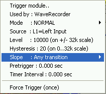
- Trigger source (in the small square = source selector, connected to the trigger block). If you don't need the trigger, disconnect the input to save CPU power. To change the source, click on the small square with the short source name (like "L1" in the screenshot).
- Trigger level, ranging from -32767...+32767 (linear steps from a 16-bit A/D converter). Can be changed in the popup menu after clicking into the trigger box, and connected to the value slider on the right side of the component window.
- Trigger slope/polarity: positive, negative, or both edges
- Trigger hysteresis: can be used if the trigger signal is noisy. Make the hysteresis value a bit larger than the noise (peak-peak value). For example, using a positive slope with hysteresis: A trigger event will only occurr, if the input voltage falls below (level-hysteresis/2) and then rises above (level+hysteresis/2). This parameter can also be connected to the slider to change this parameter on the fly.
If no signal is detected for over a second (or so), the trigger box in the circuit window turns yellow instead of green.
To use the trigger for the main waterfall, set the option "triggered spectrum" on the setup screen.
There is one sample file in the installation archive called "TrigWat1.usr" which demonstates how to use the trigger function block for the waterfall. It uses SL's test signal generator to set the scrolling speed of waterfall.
Counter / Timer (pulse- or event counter, operating in the time domain)
< T.B.D.>
The counter/timer can be configured through its context menu in the circuit window (click on the box titled "Counter"). The configurable parameters are:
- Mode:
-
At the time of this writing, only the 'Counter' mode was implemented. If
you don't need the counter (and want to save CPU time), set the Counter/Timer
mode to 'OFF' in this menu.
- Source 1, Source 2 :
-
Select the source for the counter's "main" and "auxiliary" input. If the
auxiliary input is used at all, only certain combinations are possible: L1/R1,
L2/R2, L3/R3, L4/R4, L5/R5 but nothing else.
- Trigger Level :
-
Sets the trigger level, expressed in PERCENT of 'full swing'. A trigger level
of zero means 'trigger when the signal crosses zero'. A negative value triggers
on the 'negative half wave', which makes sense if the measured signal is
mostly zero, with short negative pulses. Generally, for the best accuracy,
set the trigger level near the steepest pulse of the waveform. This would
be zero for a sine-wave like signal, and some positive value (about half
the peak pulse amplitude) for rectangular pulses.
Note: The Counter/Timer uses its own trigger module, which has nothing in common with the 'Universal Trigger Block' .
- Trigger Hysteresis :
-
Can be used to reject noise, to prevent false triggers (counts). For example,
the pulse output of a certain Geiger Counter was superimposed with a 2500
Hz sinewave, amplitudes approx. +/- 10 %, and a pulse amplitude of over 90
% (all percentages relative to "full input swing" of the soundcard's A/D
converter). To avoid counting the sinewave, the Trigger Hysteresis was set
to 10 % in this example, and the Trigger Level to 50 % .
- Trigger Slope : Rising or Falling.
-
Defines if the rising (leading) edge of a pulse shall be registered. For
simple frequency counter, it really doesn't matter. But for pulse timing
measurements (for example, to compare the PPS outputs of two different GPS
receivers), make sure you pick the right slope. Also beware that certain
soundcards (for example, the E-MU 0202) seem to invert the analog input's
polarity ! A short "positive" pulse on the analog input appeared as a short
"negative" pulse in the digitized output !
- Gate Time :
-
Number of seconds for a complete measuring cycle.
Note: The counter updates the result more frequently than the gate time. Furthermore, the frequency measurement not only uses the "number of pulses per gate interval", but also takes the timestamps of individual pulses (events) into account. Thus, even with a one-second gate time, the resolution is better than 1 Hz. But the accuracy greatly depends on the waveform (!), noise, hum, etc. Thus the requirement to set the counter's trigger level to the best possible value.
For largely dispersed signals (like the output of a Geiger counter) use a long gate time, for example 100 seconds as in the 'Geiger Counter' test application (GeigerCounter.usr).
- Holdoff Time:
-
Can be used to ignore two pulses which are very close to each other. For
example, there may be 'ringing' for a few milliseconds at the output of a
Geiger counter, or the output may be a synthetic tone burst of a few dozen
milliseconds. In such cases, use a non-zero Holdoff Time to avoid counting
the same event (particle, etc) twice.
If you don't need the holdoff function, set the holdoff time to zero. The holdoff time also limits the maximum count rate ! For example, with a 20 millisecond holdoff, it's impossible to count more than 50 pulses per second.
The counter's input (source) can be selected by clicking on the source selector, like most other elements in the circuit window.
The measured results (like frequency, total event count, etc) can be retrieved through the following interpreter functions :
-
counter.freq: returns the measured frequency in Hertz for the first channel (main input) -
The resolution depends on the counter's mode of operation, and especially
the configured gate time.
Note: The result is always scaled into Hertz (SI unit for the frequency), even if the gate time ist much longer than one second. To convert the result into something exotic like "particles per minute", multiply the result with 60 (or any other factor you like).
-
counter.event_count: returns the current value of the free-running event counter. - Read-only. Integer result. Not related to the gate time. Starts counting at zero (when the counter was started), and never resets until the program terminates.
Input Preprocessor
The input preprocessor can be used to decimate the input sampling rate before any further processing step. This may decrease the CPU load, because all later processing stages don't need to run at the 'full pace'. For example, you may only be interested in a 1 kHz wide frequency band around 77.5 kHz (including digital filtering, demodulation / decoding, etc). The soundcard would have to run at 192 kSamples/second, but the rest of the test circuit (including the spectrum analysers) only needs a fraction of that sample rate.
Besides decimation (which means reduction of the sampling rate, along with
appropriate low-pass filtering), the preprocessor can also move a signal
down in frequency, and turn it into a complex signal ... if the input isn't
already complex.
Note: Frequency shifting is also possible with SL's FFT-based filter.

Screenshot of the A/D converter block connected to SL's input preprocessor.
'L0' = left channel, directly from the soundcard, here approximately 192 kSamples/second;
'R0' = right channel, directly from the soundcard, feeds GPS sync+NMEA into the calibrator.
'L1' = output from preprocessor to the rest of the circuit with exactly 48 kS/s;
'R1': not connected due to the configuration of the Sampling Rate Detector (!)
The Input Preprocessor can be configured by clicking on its symbol in the circuit window. This will open a popup menu with the following items:
- Configure Input Preprocessor ...
-
Frequency Shift ...
-
turn off : Turns the frequency shift off.
Decimation without frequency shift is possible, the processable frequency range starts at 'zero Hertz' then.
Without frequency shift, the input preprocessor requires less CPU load, so if you don't need frequency shift at this stage, turn it off. -
turn on : Turns the frequency shift on.
The input signal will be moved down by this frequency (in Hertz) before decimation, i.e. before bandwidth limiting. - modify center frequency : Opens an edit box to modify the center frequency.
-
turn off : Turns the frequency shift off.
-
Decimate By .. ( 1, 2, 4, 8, or 16 using the old, fixed-ratio decimator)
Reduces the sampling rate, and thus the usable bandwidth, by the specified ratio.
A better job than the old, fixed-ratio decimator, possibly at the expense of a higher CPU load can be performed by the 'timestamp-driven resampler', which can not only resample the input slightly (say from 191.9876 to 192.0000 kSamples / s) but also decimate by larger fractional ratios (e.g. from 191.9876 to 48.0000 kSamples / s). The latter option can be activated by checking 'Audio Settings' (in SL's main menu), 'Audio Processing' .. '[v] use different sample rate for output', and entering '48000 S/s' (or any other sampling rate) in the field just below the checkmark. It is typically used in combination with the Continous calibration (here even 'compensation by resampling') of the input sampling rate.
The screenshot further above shows the input preprocessor when L0 is resampled (to R1), and R0 feeds the GPS signal into the soundcard. In this example, R0 is not resampled, and not routed to R1, because the sync pulse and NMEA data (from a GPS receiver) are useless 'after' the preprocessor.
- Help (on the input pre-processor) : open this page in the manual .
The preprocessor's output can also be processed
by other instances of Spectrum Lab. This helps to reduce the total
CPU load, if only a narrow frequency range shall be processed by all
running instances. For example, the first instance may receive data from
a software defined radio (like Perseus, SDR-IQ, or soundcard-based), move
down the interesting frequency range, decimate the sampling rate even further,
and then send the decimated stream to all other instances. You can use this
feature to have up to 20 (!) instances of Spectrum Lab analysing a lot of
narrow frequency bands, all fed by the first instance.
An external DLL (e.g. Audio-I/O-DLL)
can be used to distribute an audio signal 'processed' by one SL-instance to other instances,
or Spectrum Lab can act as an Audio Stream Server
providing the 'pre-processed' signal to other applications, or other instances of SL running on the same
or remote PCs.
Test Signal Generator
The test signal generator consists of...
- three independent sine wave generators (other waveforms too)
- one noise generator
- AM and FM modulator for each sine wave generator
More details about the test signal generator and its control panel can be found in this file.
Programmable Audio Filter
There are programmable filters in the center of both processing branches (for left and right channel, but they can optionally be chained as explained here). The internal functions of these filters are explained in another file. Since November 2003, there is an FFT-based filter implemented in SpecLab which can also be used as an auto-notch filter and lowpass, highpass or bandpass simultaneously.
Some general notes about the audio filter blocks inside the circuit window:
If a filter is turned off (grey color in the diagram), it is not necessarily bypassed ! To turn a filter on/off, or activate a bypass (around the filter), open the filter's control window by clicking at the filter function block in the circuit diagram. The different states of a filter look like this in the circuit window:
![]() Filter on (running), and NOT bypassed, filtered audio arrives at the right side)
Filter on (running), and NOT bypassed, filtered audio arrives at the right side)
![]() Filter off, bypassed (audio passes unchanged from left to right)
Filter off, bypassed (audio passes unchanged from left to right)
![]() Filter off, NOT bypassed (no audio arrives at the output on the filter's
right side)
Filter off, NOT bypassed (no audio arrives at the output on the filter's
right side)
Frequency Converter ("mixer")
The frequency converter is only required for special signal processing. It can be used to shift frequencies. This is achieved by multiplying a signal with the output of a sine wave generator ("local oscillator") which optionally can be a two-phase oscillator for sideband-rejecting frequency conversion.To configure one of the frequency converters, click on its symbol in the circuit window. A popup menu like this will appear:
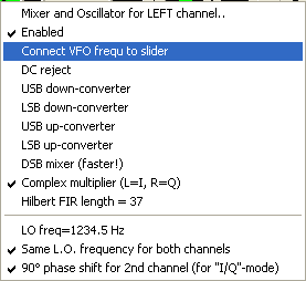
The frequency of the local oscillator can be set in the Component window. Click on the frequency display of the local oscillator and enter a new frequency, or connect the oscillator frequency to the value slider on the right side of the component window. See notes on the VLF receiver below for other ways to control the frequency.
To turn the frequency converter on (or off), left-click on its circuit symbol in the component window. As long as the frequency converter is "off", it will pass the input to the output without any change.
Notes on this frequency converter:
- There is a number of options for the frequency converters, they may be used as up- and downconverters, for either upper or lower side band, or both side bands (which is the least CPU-power consuming mode)
- There is an interpreter command to control the oscillator frequency: "circuit.osc[0].freq" can be used to read or set the oscillator frequency. This is used as VFO control for the "VLF radio", where the oscillator frequency is connected to a movable marker on the frequency scale (including audio offset).
- Multiplying a real signal (frequency f_in) with the local oscillator's frequency f_mix, (f_mix + f_in) and (f_mix - f_in) are generated. The "unwanted sideband" can be suppressed by selecting the proper mixer type ("USB down-converter", etc). These mixers for real signals require more CPU time than the "complex multiplier" because of the extra filtering.
- Multiplying a complex input signal ("I / Q"; inphase+quadrature) with a complex oscillator signal does NOT produce an extra sidebands. Instead, the signal will be simply shifted up or down in frequency, without the need for extra filtering. To use this configuration, select "Complex Multiplier" in the popup menu shown above.
- There is a file distributed with SpecLab which can turn your PC into a VLF receiver (ranging from almost DC to 24 kHz). The frequency converter is used as "LO" in that configuration, its frequency can be controlled by one of the markers on the frequency scale of the spectrum (very handy in combination with a narrow band filter!).
-
Instead of the frequency conversion in the time domain, consider using the
FFT-based audio filter, which includes
an option to shift audio frequencies up/down, and also an option to invert
frequencies (i.e. turn USB into LSB and vice versa). In many cases, the FFT-based
filter implementation requires less CPU power than the traditional
multiply-and-filter method used in these frequency converters.
Audio input and output
The input for the entire processing chain is usually the PC's soundcard, but it can also be another source or destination (an "audio server" as explained in the configuration dialog).
Output- and "cross coupling" amplifiers
After all sorts of filtering, the remaining signal amplitude at the output may be much weaker than the input signal. To adjust this without wasting much of the D/A-converters dynamic range, all signals which go into the output adders can be multiplied with an adjustable gain factor.To modify the gains, click on one of the amplifier symbols in the circuit diagram. The value slider on the right side will then be connected to the amplifier. The gain of the "normal" amplifiers is shown in DECIBELS (dB). Zero means "unity gain", positive values amplify the signal, negative values mean attenuation.
Only the "cross-coupling amplifiers" (between left and right channel) use a linear GAIN FACTOR: one means unity gain, zero turns the coupling off, and negative values can be used to SUBTRACT signals in one channel from the other. In 99.9 percent of all applications, the cross-coupling factors are set to zero, in this case their symbols are painted gray in the circuit window (="passive").
A little gimmick: With both cross-coupling amplifiers set to "-1" (which means subtract left channel from right, and subtract right channel from left), it is sometimes possible to remove the vocals from a music recording ... remember this if you are a Karaoke fan ! Why does this work (sometimes) ? Often the singer's voice is recorded more or less monophone, and mixed equally to the left and right channel, while the instruments have either a phase different or are not equally strong in both audio channels.
Alternatively, the output volume can be controlled by an automatic gain control function, which is part of every DSP blackbox.
Spectrum analyser
The spectrum analyser can be connected to the audio input or output. The output of the spectrum analyser (FFT) can be visualized as spectrum graph or waterfall, as explained here.
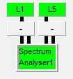
Spectrum Analyser 'input selectors' in the circuit window.
Upper row: Ch1 is connected to circuit node 'L1', Ch2 to 'L5' (green=enabled).
Lower row: Ch3 and Ch4 are not connected, and thus 'off' here (gray=disabled).
Click into one of the analyser's input blocks to select the source for that channel. The second channel can also be turned off this way (by connecting it to "nothing", which is on top of the selection list for the 2nd channel).
The spectrum analyser can be configured in a special setup screen, which can be opened by clicking into the analyser block in the circuit window (through a popup window, like for many other function blocks in the circuit window too).
The spectrum analyser can be triggered externally, using the 'universal trigger' function.
DSP Black Boxes
The "DSP Black Boxes" can be used for very special digital signal processing. They can be inserted in different places in the processing chain (shown in the Component Window ). These functions can be realized (at least):- Adder or multiplier to combine two channels (additive or multiplicative)
- Bandpass filter (often used as 'preselector' before demodulators or similar, can be used besides the more versatile FFT-based filter)
- Hard limiter (aka "clipper") can limit the wave form to a certain value
- Noiseblanker: can be used to remove pulse-type noise
- DC reject: a high-pass filter with an edge frequency of about 0.1 Hz, to remove or measure the DC component
- delay line: usable for single echo, multiple echo, crude harmonic hum eliminator
- attenuator or amplifier : use "factor" in a delay line to amplify or attenuate
- advanced hum filter (algorithm by Paul Nicholson)
- AM + FM modulators and demodulators, phase modulator, phase demodulator
- First order lowpass filter, required for wideband FM deemphasis (in the signal path after demodulation)
- Automatic Gain Control (AGC)
- Chirp Filter
The test circuit in Spectrum Lab has four black boxes (left+right channel, before and after the converters and filters). For every blackbox, an independent combination of this functions can be selected.
The properties of each "Blackbox" (oh well.. a "green box" when active..)
can be modified by left-clicking on a blackbox symbol
(![]() ) in the
component window. A
popup menu like this will appear:
) in the
component window. A
popup menu like this will appear:

Some of the blackbox components can be accessed through
interpreter commands and -functions.
Most numeric parameters can be modified through the menu shown above,
which opens an edit box. If your HTML browser isn't as bugged as
certain versions of Firefox, the 'Help' button shown in the edit box
will take you to the chapter (in this) document with details
about the purpose of the currently edited parameter.
In the following chapters some of the functions in a DSP blackbox will be
explained.
Signal processing sequence (in each DSP Blackbox)
The order in which the signal runs through a blackbox may be subject to change (or even EDITABLE in a future version), but at the time of this writing (2010-10-16) it was the same sequence as visible in the DSP blackboxes' configuration menu. For example, when active, the adder / multiplier is the first processing step in each box.
If a different processing sequence is necessary, use two blackboxes in "series". For example, use the blackbox between L1 and L2 (see circuit window) as the first stage, and the blackbox between L4 and L5 as the second stage. Remember to switch the FFT-based filter (between these two boxes) into bypass mode when the filter is not active - otherwise the signal path from L2 to L4 will be 'open' (not connected).
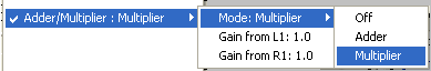
Adder or multiplier (to combine two input channels in a DSP blackbox)
This function of the DSP "blackbox" combines the input from two sources into one output signal. The sources cannot be selected freely, but are fixed:
- the first input into the adder/multiplier is the one shown in the circuit window, eg "L1" for the blackbox between L1 and L2.
- the second input is on the complementary signal path, eg "R1" for the blackbox between L1 and L2 (!) .
The gain factors can be individually adjusted through the DSP blackboxes' context menu:
Bandpass Filter (in a DSP blackbox)
In contrast to the FFT-based filter (which is not part of a DSP blackbox), independent bandpass filters can be activated in any of the DSP blackboxes. These filters are implemented as simple 8-th or 10-th order IIR filters, which can be configured through the context menu in the circuit window (left-click on a DSP blackbox, then select "Bandpass Filter" to see all possible options) . The other properties of these bandpass filters are also configured through the context menu in the circuit diagram (there is no extra dialog window for these filters).The properties of a bandpass filter are:
- Enabled / Disabled (bypassed in the signal path)
- Center Frequency in Hertz (like many other parameters, this value can be 'connected' to a slider in the circuit window)
- Bandwidth in Hertz
-
Filter Response Type :
- 10-th order Bessel (linear phase, constant group delay, but soft transition from passband to stopband)
- 10-th order Butterworth (no ripple in passband and stopband)
- 8-th order Chebyshev filters with different amounts of passband ripple (tradeoff ripple vs "sharpness" of the cutoff)
- 10-th order Gaussian filters (no overshoot to step input functions, minimum group delay)
These bandpass filters are the first (?) stage through which the signal runs in a DSP blackbox, because it was first used to limit the frequency range entering a limiter or noiseblanker (to suppress Sferics on VLF without being irritated by mains hum, and VLF transmitters).
Delay line in a DSP blackbox
The 'internal' function of a black box (if used as delay line, echo, or crude hum suppressor) is this:
- To use this as simple amplifier or attenuator:
- set "Input Factor" and "Feedback Factor" to zero, use "Bypass Factor" as gain control
- To use it as delay line with unity gain:
- set "Input Factor" to one, "Feedback" and "Bypass" to zero
- To generate a single echo:
-
set "Input Factor" and "Bypass Factor" to one (or similar) and "Feedback"
to zero.
For audio effects, an echo delay time of 0.5 seconds is a good value. - To generate multiple, slowly decaying echoes:
- set "Input Factor = 1", "Feedback Factor = 0.8" (or so), and "Bypass = 0.8"
- Suppressor for 50 Hz-hum and harmonics (from European AC mains):
-
set "Delay Time = 0.02 sec", "Input Factor = -0.7", "Feedback Factor = 0",
"Bypass Factor = 0.7"
(Factors of -1.0 and +1.0 also work, but they amplify the signal). This removes 50 Hz (1/0.02sec) and all harmonics of 50 Hz by adding the signal delayed by 20 ms to itself. Tnx Eric Vogel and Renato Romero for this idea.
In countries with 60 Hz AC mains, try 0.01667 sec (to remove 60 Hz) or 0.05 sec delay (to remove 20Hz(!) and harmonics). In the input field, instead of typing "0.01667" you may also enter "1/60", etc. The formula will calculated when you click the "Ok" button of the numeric input box.
There is also a dedicated hum filter using an algorithm by Paul Nicholson, which does not occupy the "delay line". You can activate it from the DSP blackbox popup menu. Set the "Nominal Hum Frequency" to either 50 or 60 Hz, and activate the hum filter (so it appears checked in the menu).
Advanced hum filter in a DSP blackbox
This filter is based on an algorithm by Paul Nicholson. Details were
available at http://www.abelian.demon.co.uk/humfilt/.
Note: In many cases, the FFT-based filter's "multi-auto-notch" feature
does a more efficient job, because it only removes frequencies where 'carriers'
are really present - not every harmonic of 50 or 60 Hz.
To use the old hum filter in SL, you just have to specify your AC mains frequency (50 or 60
Hz). The filter tracks this frequency within a certain range to place the
sharp nulls of the comb filter exactly on the mains frequency and its harmonics.
This only works if the mains frequency is quite stable (so not for "wandering
carriers" in a shortwave receiver, caused by free running switching-mode
power supplys). Alternatively you can provide an external source for the
AC mains frequency, for example: let the spectrum analyzer detect the precise
mains frequency (see below how to achieve this).
There is a control panel for the hum filter which can be connected to one of the four DSP blackboxes. To open the control panel, right-click on the DSP blackbox in the circuit window, point on the "hum filter" menu (so the submenu opens), then click on "Show Control Panel". On the control screen for the hum filter, you can modify...
- the nominal hum frequency (usually 50.0 or 60.0 Hz)
- the end stop for the possible hum frequency (in percent, 0.5 should be ok)
- the number of filter stages (the higher this value, the narrower the notches of the comb filter)
- the slew rate (the maximum adjustment speed for the built-in tracking algorithm)
- selection of the tracking algorithm (several versions of Paul's algorithm implemented here, plus the option to turn automatic tracking off)
- tracking cycle: Defines how frequently the current hum frequency is revised by the algorithm. A good point to start with is 0.5 ... 1 seconds.
- "Calculate current hum frequency from numeric expression": Uses SpecLab's interpreter to define an alternative source for the current hum frequency (mains frequency). See example "An alternative source.." below.
In the lower part of the window, some actual values from the tracking algorithm are displayed. They were mainly used for testing purposes, but the "Current hum frequency" may be interesting for you (dear user) as well.
- An alternative source for the current mains frequency:
-
Just let the spectrum analyzer detect the precise hum frequency. Use the
peak_f() function, like peak_f(#1, 48,
52) or peak_f(#1, 58, 62). Load the preconfigured settings "HumFi50.usr"
or "HumFi60.usr" and open the hum filter control window. The
peak-frequency-detection routine is entered in the edit field under the checkmark
"Calculate current hum frequency from expression". Note that the 1st channel
(#1) of the frequency analyzer (which feeds the waterfall) is connected to
the INPUT of the DSP blackbox (labelled "L1"). Be careful not to connect
this channel to "L2", because the 50 Hz / 60 Hz signal is notched in the
output of the DSP blackbox !
For accurate tracking we need a good SNR of the 50 Hz / 60 Hz line, otherwise the interpolation in the peak_f function is severely degraded. If your VLF antenna does not pick up enough hum, switch the program to "stereo" mode and use the second input of your soundcard as an auxiliary hum input. Use an insulated piece of wire as "hum antenna", tied around a power cable or similar. Connect one input of the spectrum analyzer to this auxiliary hum input. The result can be stunning if you are listening to VLF with the soundcard !
Hard Limiter in a DSP blackbox
The limiter simply clips the waveform to one of two possible adjustable "maximum" values:-
Clipping level A :
This limit doesn't depend on the signal amplitude itself. It is entered in "dB over full scale". A "full scale" value of 0 dB is the point on which clipping takes place in the A/D, and in the D/A converter. Typical settings for this parameter are -3 to -6 dB "above" full scale (note the negative dB values; the limits are actually always below full scale). -
Clipping level B :
This limit is relative to the average signal amplitude. 3 dB means "clip anything which is 3 dB above the average signal level".
The program will automatically use the lower of these two limits.
When opening the submenu "Hard Limiter" in the popup menu of a DSP blackbox,
the program may show a message like this (if the limiter is enable) :
-
"Signal is 10.4 dB below clipping(A); avrg = -12.3 dBfs" .
This means (for example) :
-
At the moment, the input signal (to the blackbox) is 10.4 dB below
the lower of the two clipping levels,
the lower is clipping level A (see above), and the average input signal is 12.3 dB below full scale.
To adjust the two clipping levels (A and B), these parameters can be connected
to the vertical slider in the circuit window.
Select "Hard Limiter"..."Clipping Level A" (or B) in the blackbox menu, and
when prompted for the new value, set the option "Connect to slider".
- Hint:
-
Connecting the Hard Limiter in front of the digimode terminal may help under
certain (special") conditions, for example with the PSK31 decoder.
Also, it helps when listening to shortwave radio stations if the signal is affected by static crashes. Because the signal first runs through the limiter (before it enters the optional AGC), the deafening effect can (impact on the gain control) be reduced. Unlike the Noise Blanker (see below), the Hard Limiter doesn't punch a "hole" into the signal. A combination of the Limiter and the Noise Blanker is possible, but makes little sense.
Noise Blanker in a DSP blackbox
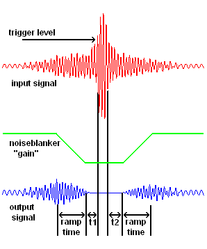
The noise blanker can be used to suppress pulse-type noise, as often caused by electric fences, switches, and thunderstorms. It basically works like this:If the signal rises above the average by more than a certain amount (expressed as "Trigger peak / averag" in decibel) within a short time, and only for a short duration, the "gain" of the noiseblanker will be reduced by this amount. The gain reduction will have smoothed ramps (rising and falling edges) to avoid AM sidebands in the output signals.
The adjustable parameters of the noiseblankers are:
-
Ramp time
Set to 0.01 seconds by default, to reduce sidebands caused by the blanker's amplitude modulation. If the noise pulses are very short (typically shorter than 10 milliseconds), reduce this value. Remember, you can connect (almost) all parameters to the value slider in the circuit window. -
Trigger level ( relative to a an average, in decibels)
Defines the level at which a blanking pulse shall be started. The average value is taken from the input signal, full-wave rectified, and low-pass filtered. Thus values below 3 dB are useless - at least for a few very special cases. Don't make this value too low, to prevent false triggers. 20 dB (above average) seem to be a good value for listening on longwave. With this value, the effect of "QRN" (static crashes) on a waterfall display can be reduced also. It takes some experimentation to find the best value for a given purpose - remember the value slider.. and the possibility to plot the noiseblanker's currently measured average level as explained further below. -
Pre-trigger blanking time (t1), post-trigger blanking time (t2) :
Can be set to zero in most cases. In some cases (depending on the 'waveform', see red graph in the diagram), blanking can actually start a short time (t1) before the trigger threshold is reached, and extend a short time after the signal falls below the trigger threshold. Quite annoying for listening, but it may help to reduce the unwanted energy from sferics in weak signal analysis (with very long FFTs, where a slightly longer gap in the input matters less than the 'burst noise' energy). -
Average detector time constant(s)
This is the lowpass filter's time constant (in seconds) for the average value. Typically a few seconds. Example (VLF, sferic blanking): 5 seconds. There are actually two time constants:
the RISE time constant is used while the rectified signal
exceeds the average; the DECAY time is used otherwise.
For weak-signal work, it helps to use a slower RISE- than DECAY-time for averaging, to avoid upsetting the average by sferics.
Note: In some cases, it helps to run the signal through a bandpass filter before it enters the noiseblanker (or similar non-linear processing stage). For example, if the input from the receiver (soundcard, SDR, etc) contains strong signal which are *not* impulsive noise (and thus shall not trigger the noiseblanker), a bandpass filter which rejects the non-impulsive noise helps to prevent false triggers of the blanker, and allows setting the trigger level to a lower value. In a VLF radio experiment, the combination of a bandpass filter followed by a noiseblanker was used to remove sferics (distant lightning discharges) before the signal entered the spectrum analyser, which used a very large FFT to dig a weak but coherent signal out of the noise.
To test the noiseblanker (and find the best settings for a given type of noise),
some of its internal state variables can be read via the built-in interpreter,
and thus can be watched / plotted:
- blackbox[N].nbl.avrg (where 'N' is the DSP blackbox index, 0..3):
The noise blanker's current average level (for the dynamic trigger level), "rectified and low-pass-filtered amplitude", not a logarithmic unit.
Since digital samples within Spectrum Lab are normalized from -1 to +1 internally, the expectable value range of the noiseblanker average level is zero (complete silence) to 1.0 (clipping level of the A/D converter). - blackbox[N].nbl.avrg_dBfs
Similar as blackbox[N].nbl.avrg, but the unit is "decibel over full scale" (logarithmic scale).
DC Reject / DC measurement (in a DSP blackbox)
Similar to a 'coupling capacitor' in an audio amplifier, a signal's DC component can be removed. This is achieved by a simple 1st-order highpass filter with a lower corner frequency of approximately 0.1 Hz .When enabled, the (removed) DC offset can be read (measured) with the interpreter function 'blackbox[N].dc_offset' .
Modulators and Demodulators in a DSP blackbox
In each of the four DSP blackboxes, there is a "modulator"/"demodulator" function for either amplitude-, frequency- or phase-modulation. It can also be used for frequency conversion (like the multiplier, but with sideband rejection using the Weaver method).Depending on the type, you must specify:
- center frequency
- modulation bandwidth
- carrier amplitude
- modulation factor
Possible types are selectable through the blackboxes' specific menu (left-click on the symbol in the circuit diagram... see below):
- Amplitude modulator
- Frequency modulator
- Phase modulator
- Amplitude demodulator
- Frequency demodulator
- Phase demodulator (note: the output is scaled to -180 to +180 degrees, which may change in future revisions, when "everything" will be normalized to +/- 1.0)
To modify the type or properties of a modulator/demodulator, click on the DSP blackbox in the circuit window to open a DSP popup menu.
Wideband FM reception
For wideband FM, activate the FM deemphasis unit (which is nothing more than a digital implementation of a simple RC lowpass filter). For north american FM stations, use a time constant of 75 microseconds. For the rest of the world, use 50 microseconds. The configuration "UKW_FM_Demodulator_SDR_IQ.usr" or "UKW_FM_Demodulator_Perseus.usr" can be used as a starting point to receive FM broadcasters with one of these software-defined radios. In these configurations, the left part of the spectrum analyser shows the input spectrum (before FM demodulation), while the right part shows the demodulated baseband signal. The FFT-based filter is used as an IF filter in the above configurations. The IF bandwidth can be adjusted with the blue frequency marker in the left part of the spectrum (it is actually one of the programmable frequency markers). Stereo reception and special functions like RDS decoding is not possible (yet ?). But you may be able to see the stereo (L-R) subcarrier, double-sideband modulated around 38 kHz, and the 19 kHz stereo pilot tone at 19 kHz in the right half of the spectrum display.Using a normal soundcard (and a VHF downconverter of course) to receive wideband FM is impossible due to the lack of necessary bandwidth. Only soundcards with a sampling rate of 192 kHz can be used to receive FM with just a simple downconverter.
Automatic Gain Control (in the DSP blackboxes)
For listening to certain signals comfortably, without damaging your ears if the signal suddenly gets too strong due to QSB (fading), you may want to have a constant output level (on average) despite changing strength of the input signal. This is especially helpful when using SpecLab as the last stage of a radio receiver, or as a complete VLF or LF receiver. Use the AGC (automatic gain control) which is the last processing stage within a DSP blackboxes.To turn the AGC on or off, or switch between "slow, mid, and fast" mode, use the DSP popup menu in the circuit diagram, and point to the "Automatic Gain Control" entry. A submenu with the following entries will open:
-
Mode
allows to switch the AGC on/off or select the speed. The "slow" AGC is the most comfortable mode for longwave- and shortwave listening. -
Target Level
defines the "target" average level of the AGC'ed signal, expressed in "decibel before clipping takes place". For sine-like signals, a value of -3 dB is ok, for other pulse-like signals which require more headroom, set the Target Level to -6 dB or even less. -
Min. Gain, Max. Gain
can be used to limit the gain range of the AGC. If there is "no signal at all", you may want to limit the gain to avoid hearing a hissing broadband noise in your speakers. A maximum gain between +60 and +80 dB is usually sufficient, but this depends greatly on your application. -
Momentary Gain
shows the momentary gain of the AGC control loop. If you connect this value to the slider in the circuit window (by checking "connect to sllider" mark in the edit window after selecting this menu), you have a "living" display of the current gain depending on the averaged input amplitude.
Chirp Filter (in the DSP blackboxes)
For experiments with a chirp sounding, or a chirped backscatter radar, a chirp filter was added to all of the four DSP blackboxes.Details about the chirp filter are in a separate document (chirp_filter.htm) .
Sampling Rate- and Frequency Offset Calibrator
The small blocks labelled "SR cal" and "FO cal" in the circuit diagram show the current status of the sampling rate- and frequency offset calibrator. Clicking on one of these blocks opens a control panel where the properties of the calibrators can be edited, etc.More info about these frequency calibrators are explained in another file.
Interpreter commands for the test circuit
- blackbox[N].xxx
-
Access to some of the DSP blackbox components.
"N" is the blackbox index:
0=blackbox near left input, 1=blackbox near right input, 2=before left output, 3=before right output.
The following blackbox components can be accessed this way (most read- and writeable):
blackbox[N].agc.mode: 0=off, 1=fast, 2=medium, 3=fast, 4=custom (see attack,decay)
blackbox[N].agc.tgt_level: target output level in decibel
blackbox[N].agc.min_gain: minimum gain of the AGC block in dB
blackbox[N].agc.max_gain: maximum gain of the AGC block in dB
blackbox[N].agc.mom_gain: momentary gain of the AGC block in dB, read-only !
blackbox[N].agc.attack: custom-defined attack speed, arbitrary unit. 1.0 is "very fast", 0.01 is medium speed
blackbox[N].agc.decay: custom-defined decay speed, same arbitrary unit as the attack speed
blackbox[N].delay.sec: approximate delay line lenth in seconds. The actual delay will be a multiple of sample intervals.
blackbox[N].delay.enabled: 0 when disabled, 1 when enabled.
blackbox[N].delay.input_factor: 0..1 . See diagram of a delay line.
blackbox[N].delay.feedback_factor: 0=no feedback .. 1=full feedback (causes oscillation). See diagram of a delay line.
blackbox[N].delay.bypass_factor: 0=no bypass .. 1=full bypass. See diagram of a delay line.
blackbox[N].dc_offset: reads the current DC offset voltage, detected by the DC-rejecting function.
blackbox[N].nbl.avrg: returns the noiseblanker's current average level (linear scale, not "dB"), which affects the threshold aka 'trigger level'.
Note: There may be more noiseblanker-related functions here.
- circuit.osc.freq
-
Reads or sets the oscillator frequency (in Hertz) for the
frequency converter.
If you use the stereo mode and two different oscillators:
circuit.osc[0].freq is for the LEFT audio channel,
circuit.osc[1].freq is for the RIGHT audio channel.
Example: VFO control for the "VLF radio",
- sr_cal.xxxx
-
Sampling rate calibrator.
- fo_cal.xxxx
- Frequency offset calibrator (or "drift detector")
Last modified : 2021-05-15
Benötigen Sie eine deutsche Übersetzung ? Vielleicht hilft dieser Übersetzer - auch wenn das Resultat z.T. recht "drollig" ausfällt !
Avez-vous besoin d'une traduction en français ? Peut-être que ce traducteur vous aidera !