
Digital Filters
The digital filters are embedded in Spectrum Lab's test circuit. There is one 'large' (FFT-based) filter for each of the two possible channels, but both channels can be combined into one long processing chain. A filter can be used for many purposes. This chapter mainly describes the FFT-based filter. In addition, each of Spectrum Lab's four "DSP Blackboxes" can operate as a simple IIR bandpass filter (see links below).
Contents of this document
-
FFT filter (with frequency inverter, -shifter,
autonotch, denoiser, various filter types and
plugins)
- Control panel (for the filter)
- Controlling the filter via SL's main frequency scale
- Frequency Conversion ("pitch shift")
- Frequency Inversion (USB <-> LSB pitch shift")
- FFT-based autonotch (automatic notch filter)
- I/Q processing (with the FFT filter)
- FFT-filter used as I/Q modulator (to generate SSB signals for I/Q-based transmitters)
- FFT-filter used as I/Q demodulator (demodulate SSB from a frontend with I/Q output)
- FFT Filter Plugins
- Filter implementation
- Starting and stopping the filter
- Testing a filter
- DSP literature
- Interpreter commands for the digital filters
See also: Spectrum Lab's main index, 'A to Z', circuit window, comb filter, simple IIR bandpass filters in each DSP blackbox .
FFT filter
The FFT-based filters are basically FIR filters, but the filtering is not done in the time domain. The input signal is transformed from the time- into the frequency domain (using the FFT), the spectrum multiplied with the filter's frequency response, and the result is transformed back into the time domain (using the inverse FFT). Though this sounds more complicated than the classic FIR implementation in a DSP, it's actually much faster if the filter has a high order (=a large number of coefficients). And it offers some special options -see the list of operations below- which are otherwise difficult to achieve.
With an FFT-based FIR filter, you can realize increadibly steep transitions, extreme stopband attenuation, and a linear phase - which is almost impossible with a simple FIR- or IIR filter. Since 2006, the filter can additionally move frequencies up or down, and turn USB into LSB (upper / lower sideband). The following list shows the sequence of the operations performed inside the filter:
- Transform a block of samples from the time- to the frequency-domain (FFT)
- If loaded and configured as the "first step": Pass the transformed data to the FFT-filter plugin
- Move frequencies down (option, one of the first steps in the frequency domain when converting "down")
- frequency-selective limiter (optionally)
- automatic multi-notch filter (to remove "steady carriers", optionally)
- denoiser (option.. using spectral subtraction)
-
FILTER (always active, may be bandpass, lowpass, highpass, bandgap, or
custom-type).
In the frequency domain, this is just a multiplication of the samples with the filter's frequency response. - Move frequencies up (option, last step in the frequency domain when converting "up")
- If loaded and configured as the "last step": Pass the transformed data to the FFT-filter plugin
- Transform back from frequency- to time domain (inverse FFT)
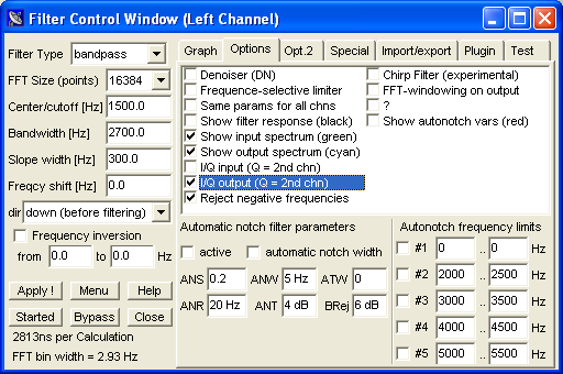
There is an extra tabsheet for the two FFT filters in the filter control window. If you want to use the FFT filter as a simple lowpass, highpass, bandpass or bandgap, select the filter type from the combo box, enter the center- or cutoff frequency and -possibly- the bandwidth in the edit fields (advanced users can also set these parameters through interpreter commands instead of defining them on the panel shown below). One example for controlling the FFT-filter through the interpreter is the "SAQ VLF Receiver" (software defined radio for the VLF band, 3 to 24 kHz).
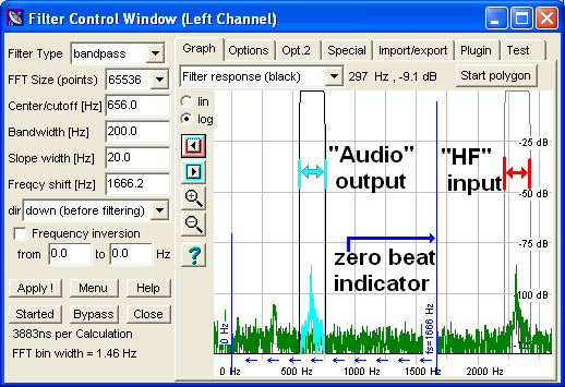
(screenshot "FFT filter control panel")
Controls and Options for the FFT-based filter
The following controls (input fields, selection combos) and options (mostly checkmarks) are located on the main tab of the filter control panel:
- Enabled: If checked, filter block uses the FFT filter (otherwise conventional filter in the time domain)
- Filter type: Select lowpass, highpass, bandpass, band reject or custom here. For the "custom"-type filter, you can draw the frequency response with the mouse in the lower right part of this window. Different editing modes are available ('point', 'polygon', 'smoothing').
-
FFT size (points): Defines the filter's frequency resolution:
frequency resolution (FFT bin width in Hz) = 0.5 * sample rate / FFT size .
For steep edges, very narrow notches, etc use the highest possible value. Downside: The larger the FFT size, the longer the delay introduced by the FFT filter. The FFT size also affects the 'reaction speed' of the autonotch filter. Suggestion: Play around with these parameters to find the best value for your application.
See also: Relation between sampling rate, FFT size, and FFT bin width for the spectrum analyser. - Center/Cutoff: For bandpass and band reject filters, enter the center frequency here. For lowpass and highpass, this is the frequency of the -3dB cutoff point.
-
Bandwidth: For bandpass and band reject only. Defines the bandwidth
(in Hertz) between the -3dB points.
Note: You can connect the center frequency, the bandwidth control, and the optional shift frequency to SL's frequency markers. This way, you can easily change these values by moving the diamond-shaped frequency markers on the frequency scale. Details in one of the following chapters. -
Slope width: Width of the filter skirts in Hertz. You may find
that the steepest possible filter is not always the best - for example, for
a morse code filter a smooth filter may "sound" better than a filter with
extremely steep edges.
In fact, the slope width (aka transition width between passband and stopband) must be a multiple of the filter's FFT bin width. The FFT bin width depends on the sampling rate divided by the the FFT size; it is displayed in the lower left corner of the filter control window (see screenshot above). To avoid audible artefacts, make the slope width at least three times larger than the FFT bin width. - Frequency shift / direction: Shift frequencies up or down within the FFT filter. More info in these notes about the FFT-based frequency converter. The shift value (offset in Hz) is displayed as a blue vertical line in the graph; the direction as arrows (down=arrow left, up=arrow right). If the frequency shift is enabled, the filter fresponse will be shown in the graph (see below) in black colour at the baseband frequency, and in gray colour at the "high" (converted) frequency. If the direction is "UP", the input signal is filtered first, and frequencies shifted afterwards. If the direction is "DOWN", the frequencies are shifted first, and filtered afterwards. This simplifies the task of switching between transmit and receive, if SL is used as a software-defined radio.
- Frequency inversion range: Mirrors all frequencies (FFT bins) in a certain frequency range. Can be used to convert the upper side band into lower side band and vice versa. Note that due to the sequence of operations inside the FFT-based filter, this happens in the baseband (=low frequency range). The inversion range is displayed as a double-ended green/orange arrow in the graph.
- Started / Stopped : This button starts / stops the filter. If the button shows "Started", the filter has been started (and clicking the button stops it). If the button shows "Stopped", the filter has been stopped, and the next click will start it again. In geek-speak, it's a "toggle button".
- Bypass : This button toggles the 'bypass mode'. When bypassed (regardless of the filter being "on" or "off"), a signal entering the filter (label L3 or R3 in the circuit diagram) will leave the filter unchanged (at label L4 or R4 in the circuit diagram). It makes sense to run a filter in 'bypass' mode if the filter is only used for special kinds of signal analyses, for example by means of a filter plugin. But normally, if you don't need the filter, turn it off to save CPU power. This button also shows the current state: "Bypassed" means the filter is bypassed, "Bypass" means "not bypassed at the moment, but a click on this button will switch the filter into 'bypassed' mode.
- Apply : This button is rarely used, because changing something in most of the edit fields on this panel will have an immediate effect. In earlier versions of the program, the 'Apply'-button had to be clicked after typing a new center frequency, bandwidth, shift value, slope width, etc in the edit fields mentioned above.
On the "Graph" tab of the FFT-filter control panel, the most important parameters are displayed in graphical form and can be modified with the mouse (by clicking into the graph). Some of the graphic elements can be turned on and off on the "options" tab (next paragraph). Controls on this tabsheet are:
-
Selection combo (box in the upper left corner): Select what
you want to edit with the mouse (left button) in the graph. You can modify
the frequency response, the limiter threshold levels, and some other parameters.
-
The combo box in the right above the graph (with "Points", "Polygon", "Smooth")
can be used to toggle between "single point" and "polygon drawing"
mode. In Polygon mode, the program calculates a linear interpolatation
between two points, which helps to draw a completely new curve, like this:
- Select "Polygon" in the combo box.
- Click on the first point in the curve area (usually beginning at the left side of the graph)
- Click on the next point in the curve area (usually further right, i.e. on a higher frequency)
- Temporarily move the mouse outside the curve area to begin a new segment with the next click.
The program will fill the curve with a linear interpolation between the two clicked points. This works for different types of graphs in the diagram (custom filter response, threshold levels, as selected in the combo box on the left side).
After editing the curve as explained above, kinks can be remoted by switching from 'Points' or 'Polygon' editing to 'Smooth'. In that mode, two sliders appear on the left side of the window. These sliders control the normalized cutoff frequency, and the transition width ("steepness") of a lowpass filter which will be applied to the custom filter response, or any other editable curve. A cutoff value of zero means 'DC' (sets all points of the curve to the average value), a cutoff value of one means 'no lowpass at all', and returns all points of the curve to the original values.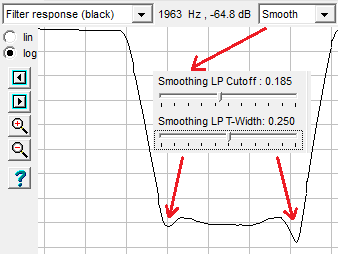
- "Lin" / "Log" : These radio buttons select linear or logarithmic display. Logarithmic is often the better choice due to its large dynamic range. Too low levels can not be seen on a linear scale. The logarithmic scale is in fact "decibel below the clipping point", as in most other parts of Spectrum Lab.
- Other small buttons just left to the graph area can be used to zoom into the graph, and to scroll the displayed frequency range left or right.
The black graph shows the filter response in the baseband, the gray graph is the same but shifted up or down, depending on the frequency-shift settings. Together with the option 'show input spectrum', this feature can be used like the VFO in a software-defined radio.
Less often used controls are on the "options" tab:
- Autonotch: Adds an multi-frequency autonotch to the FFT filter. Function described in one of the next chapters.
- Denoiser: A simple denoiser, uses "spectral subtraction" of a constant value from all FFT bins (magnitudes in the frequency domain).
- Frequency-selective limiter : An experimental "signal limiter". All spectrum lines which exceed a certain, individual level (painted as red line into the graph) will be limited to just that level. This may be helpful to reduce man-made interference (strong, steady carriers) in a spectrum where you are interested in the weaker components (like whistlers and other noise-like signals in natural radio recordings). To set the proper threshold levels, turn on the display of the momentary input (green line), and then set the signals in the diagram (using the mouse in "polygon" mode). Everything below the threshold will not be affected (in contrast to the multi-frequency automatic notch, which always rips some of the wanted signals apart). Thanks to Renato Romero for the suggestion ! To listen to the effect of this filter on various kinds of noise, load the configuration file FFT_lim1.usr (it uses the generator as an artificial noise source, turn the generator off to listen to real-world signals).
- Same params for both channels: Only important for stereo mode. If checked, the 2nd channel uses the same filter parameters at the 1st.
- Show input spectrum: If checked, the filter's frequency response is shown in the spectrum graph in the main window (dark green).
- Show output spectrum: If checked, the filter's frequency response is shown in the spectrum graph in the main window (cyan colour).
- I/Q-Input: Inphase and Quadrature input to the filter. Can be used for image-cancelling direct conversion receivers (a bit like "software defined radio") as explained in another chapter. In I/Q-mode, the filter can process negative and positive frequencies, which gives a useable bandwidth of almost 96 kHz for a 96-kHz sampling rate.
- I/Q-Output: Inphase and Quadrature output from the filter. Can be used to drive single-sideband transmitters with little overhead (but beware the caveats resulting from non-perfect soundcard outputs !). I/Q processing is explained in another chapter.
- Frequency response file: Name of the file in which the frequency response of the "custom"-type filter is saved.
- autonotch speed: A relative measure for the 'speed' of the autonotch filter. A value of 1.0 would mean 'immediate reaction' so the signal will virtually be subtracted from itself. A value of 0.0 means ultimately slow reaction, in fact the notches won't change at all. For listening purposes, 0.02 .. 0.2 are good values, and 0.1 is a good starting point for experimentation.
- denoiser level: This level (relative to 0.0dB which is the soundcard's clipping point) will be subtracted from all magnitudes in the frequency domain. Because white noise is equally distributed over the spectrum, the impact of this subtraction is significantly larger than on coherent signals. A good starting point is setting the denoiser level slightly above the noise level, for example -60dB. Too high values for the denoiser level (above - 40dB) cause funny sounding noises and make human voices unreadable.
Notes:
- The FFT used in these filters is not affected by the "FFT settings" for the spectrum display. The filter is an encapsulated function block which has no connection to the spectrum analyzer (unless you use some tricky programming with SpecLab's built-in interpreter).
-
On a 1.7-GHz-Pentium 4, with stereo processing at 44.1 kHz sample rate, the
FFT filters consume about 6 % of the CPU power.
Special frequency ranges for the FFT-based filter
Besides the usual low-, high-, and bandpass filters, frequency shifter, and notch filters,
the FFT-based filter also supports special operations in certain user-defined frequency ranges.
Those frequency ranges can be entered in a table on the 'Special' tab in SL's filter control window.
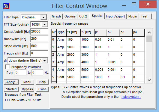
The type of operation performed inside a certain frequency range is specified as an upper-case letter
in the 'Type' column. In columns 'f1' and 'f2', enter the frequency range in Hertz ("from", "to").
The meaning of the other columns ( parameters 'p1' to 'p4' ) depends on the type, as listed below:
| Type | p1 | p2 | p3 | p4 |
| A(mplify) | linear gain factor for first bin (1=pass-through; -1=invert, etc) |
factor for last bin (linear interpolation when not equal to p1) |
||
| S(hift) | factor for shifted bins (1 for neither gain nor attenuation) |
factor for old source (0 to remove original, non-shifted signal) |
factor for overlapped destination (0 for no overlap in the destination range) |
- Note:
- Frequency ranges may overlap. If they do, the processing sequence matters. The sequence can be modified
by grabbing the 'Nr' cell with the left mouse button, and moving it up or down
to the new position in the table.
Controlling the filter via SL's main frequency scale
If the FFT-based filter is used as a simple bandpass filter, with optional frequency shift,
the most important parameters can alternatively be controlled on Spectrum Lab's main frequency scale :
           |
           |   'zero beat' marker or 'carrier frequency'


             __
           _/   lower cutoff frequency


           __
             \_  upper cutoff frequency
To show/hide these controls in the main frequency scale, right-click into it, then select 'Frequency Scale Options'
in the context menu, and check/uncheck the item 'show filter passband(s)'.
(screenshot of main frequency scale with filter passband display / controls)
The control elements for the first(*) filter channel (usually connected to the "left" audio output) are painted in blue .
The control elements for the second filter channel ("right" audio output) are painted in red .
Moving the mouse over one of the three important parameters will highlight it on the frequency scale (bold instead of thin lines),
and show the current value near the mouse cursor (see screenshot above; ).
Press and hold the left mouse button to drag the currently selected parameter.
With the mouse pointing into the middle of the passband, all three parameters (zero beat frequency, and both edge frequencies)
can be shifted by the same amount; similar to the VFO of a classic USB/LSB/CW receiver but limited to the audio passband.
A double click on the passband indicator in the main frequency scale opens the filter's extra control panel,
where more filter parameters can be modified (see previous chapter).
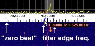
For USB (upper sideband) reception, the 'zero beat' marker must be on the left side, below the audio passband:
           |    ______
           |  _/      \_

          (filter controls set for USB reception.
           'zero beat' marker on the LEFT side)
For LSB (lower sideband) reception, the 'zero beat' marker must be on the right side, above the audio passband:
               ______    |
             _/      \_  |

          (filter controls set for LSB reception.
           'zero beat' marker on the RIGHT side)
Depending on the relative position of the 'zero beat' marker, Spectrum Lab will automatically invert the frequencies in the audio passband as necessary. The effect can be seen on the filter's extra control panel (see links below).
- (*) About filter channels:
- Filter channels can be activated/deactivated on the filter control panel (see link below).
To select a different filter channel, use the 'Menu' button in the lower part of the filter control panel, or click into the filter block in SL's Component Window ("circuit").
Only the passband of enabled and not-bypassed filters will be displayed on the main frequency scale.
FFT-based frequency conversion ("pitch shift")
Unlike a classic frequency converter (also available in SL), the FFT-based filter can only shift frequencies by multiples of an FFT bin width. The longer the FFT, the finer the stepwidth for this kind of frequency conversion.
If frequencies shall be moved DOWN, the conversion takes place as the first processing step. If frequencies shall be moved UP, it happens as last processing step. This the filter response, frequency inversion range, etc always remain at 'baseband' frequencies - regardless of the shift value. This simplifies switching from receive (=move frequency DOWN) and transmit (=move frequency UP), if the FFT-based filter is used as the core for a software-defined radio.
For convenience, the frequency shift can be controlled by any of the frequency
markers ("diamonds") on the main frequency scale, so you can move the marker
with the mouse for tuning like in a software-defined radio. More details
on this are in the chapter 'Interpreter commands
for the digital filters'.
Alternatively (added in later versions), the frequency shift can also be controlled
by dragging an indicator on SL's main frequency scale as explained here.
FFT-based USB / LSB conversion ("frequency inversion")
<ToDo> (works, but subject to change)
FFT-based automatic notch filter
The autonotch in the FFT-based filter basically works as follows ("special options" explained later) :
- Convert a block of samples from the time domain into the frequency domain, using the FFT. Let's call the result "FFT bins". Each bin is typically just a few Hertz wide, depending on the filter's configurable FFT Size.
- Calculate the powers from all FFT bins.
- From the powers of current FFT bins, calculate "slowly average". The autonotch speed parameter is used in this step.
- Compare the power of each (averaged) FFT bin with its neighbours. If the bin exceeds the average power of its neighbours (say 10 bins to the left and the right), set this bin in the complex spectrum (and a few bins to the left and the right, depending on the configuration) to zero.
- Multiply the complex spectrum with the filter coefficients (like in normal mode without autonotch, for bandpass / lowpass / highpass function).
- Convert the complex spectrum back into the time domain, using another ("inverse") FFT.
The sample blocks use a 50 percent overlap (from the previous block), and
a cos^2 window, to avoid aliasing effects which would cause an ugly low-pitched
clicking sound. If you have the C++ sourcefiles, you can find more details
about the windowing function in the file FftFilter.cpp (available
on request).
Options for the FFT-based automatic notch filter
The automatic (multi-) notch filter can be configured on the "Option"-tab of the filter control panel. Besides this, 'fixed' notches can be inserted into the filter response by using a 'custom' filter response (manually edited curve) or by activating special frequency ranges with a 'gain' of zero.
Due to the limited space on that panel, some parameters are only labelled with cryptic abbreviations.
- AFL: Autonotch Frequency Limit (in Hertz)
- Allows to limit the frequency range for the automatic notches. Set this range to "0 ... 0 Hz" to let it operate in the entire frequency range. If, for example, you only want to remove constant "carriers" between 45 and 5000 Hz, enter that range here.
- auto NW: Automatic Notch WIDTH (checkmark)
- If this (experimental) option is enabled, the automatic notch filter will choose the width of each notch automatically. Otherwise, the notch width is defined by the "ANW" field in Hz - see below.
- ANS : Automatic Notch Speed.
- This dimensionless parameter defines the relative speed" of the adaption of the automatic notches to match the received signal. In other words, it defines "how fast" new signals with an almost constant frequency and amplitude will be removed, and how fast notches on "clear" frequencies will disappear. The usable range is zero to one, a typical setting is 0.1 .
- ANW : Width of a single notch for the automatic notch filter in Hertz.
- Only has an effect if the option "auto NW" is *not* checked.
- ATW : Autonotch Transition Width (unit: number of FFT frequency bins)
- This parameter can be used to make the transition between stopband and passband (for each notch) smoother. In some cases -for example if a *very* strong signal is notched away- a smooth transition can reduce the amout of "filter ringing", even though the FFT-based filter is an FIR filter (not an IIR filter) by design.
- ANR : Autonotch Region width (unit: Hz)
-
To decide where to place a notch, the algorithm compares each bin power with
the average of its neighbours. This parameter defines the "number of neighbours",
but as a width in Hz, not as a number of frequency bins. However the algorithm
look at a minimum number of 3 neighbours (on each side), so this parameter
may be ignored if the FFT size is too low. Note that the FFT bin width (in
Hz) is displayed near the lower left corner of the filter control panel.
As a rule of thumb, make the region small enough so the 'wanted' signals don't get wiped out. If, for example, a wanted signal has a bandwidth of 100 Hz (due to its modulation), a region width of 20 Hz ensures that the signal does *not* get wiped out.
On the other hand, make the region wide enough so 'unwanted' signals will be removed. For example, the AC mains frequency (and its harmonics), or the QRM emitted by a switching mode power supply may be "drifting", effectively widening the bandwidth to a few Hz. If the region is too small, and the unwanted signal too "wide" (spectrally), the ratio between the bin power and average of its (few) neighbours will be too small to reach the autonotch threshold value (ANT, see below). - ANT : Autonotch Threshold (unit: dB between bin power and the mean power within the 'region width' (ANR).
- Only signals exceeding this value will be notched out.
- BRej : Burst Reject Threshold (unit: dB between momentary total power and average total power)
-
This parameter is used to avoid "irritation" of the algorithm from short,
strong bursts of noise (like Sferics in the VLF spectrum).
An explanation by Paul Nicholson (who suggested this algorithm - thanks Paul):
To avoid upsetting the filter settings every time a loud sferic or lightning crash comes in, we only revise the notch settings when the total signal power in this frame compared with the average total power in recent frames is below a threshold.
The 'Burst Reject Threshold' parameter was originally a power ratio of two, i.e. 3 dB difference between momentary and average power (over the entire input spectrum).
I/Q processing with the FFT-filter
The FFT-based filter can operate in I/Q-mode. I/Q means "Inphase" and
"Quadrature" channel. Search the web on "I/Q signal processing", or
just "quadrature signals" in the context of digital signal processing. A
few notes on how to use the spectrum analyser in I/Q mode is
here. Some applications
of the FFT-filter in I/Q-mode are described in the chapter about
image-cancelling
direct conversion receivers.
Basically, the filter processes complex values in this mode. In fact, it's
complex but not complicated !
The following combinations can be selected on the Options tab of the FFT filter control panel:
-
I/Q input *and* I/Q output
In this mode, both in- and output are complex samples. The filter response covers negative and positive frequencies. -
I/Q input + real output (no I/Q output)
The input covers negative and positive frequencies, but only positive frequencies are sent to the output (with one channel). Negative frequencies can be processed though, because the FFT-based filter allows shifting frequencies from the negative part of the spectrum into the positive part, with optional mirror for the passband. Typically used as the demodulator in a single-sideband receiver with I/Q-frontend. -
real input + I/Q output
Typically used in single-sideband exciters. The "real input" may be from a microphone, the "I/Q output" may go to an image-rejecting modulator like this one.
For details, see chapter FFT-based filter as I/Q modulator (to generate SSB signals).
-
real input + real output
This is the old, default mode without I/Q processing. The filter doesn't care for negative frequencies in this mode, so the graph only shows positive frequencies.
FFT-based filter as I/Q modulator (to generate SSB signals)
With the configuration shown below, the filter generates an I/Q output for the soundcard. Such a signal can be used to drive single-sideband transmitters without the need for a broadband 90° audio phase shifter.
The filter passband (audio frequency range) shown here is adequate for SSB voice transmission.
The filter's output delivers the I (inphase) component on one channel, and the Q (quadrature) component on the other channel. The signal path (inside SL) can be seen and modified in the circuit window. Note that the connections in the vincinity of the filter will be automatically modified: Instead of two independent filters (one in the upper "L" branch for the left audio channel, one in the lower "R" branch for the right audio channel), there is only one active filter in this mode, with two inputs, and two outputs.
The output (I/Q signal) can be checked with the spectrum analyser, configured for complex input.
For example, see the configuration 'FFT_Filter_as_IQ_Modulator.usr' (contained in the SL subfolder 'configurations'). Make sure the soundcard output levels (also the balance) is properly set, otherwise the suppression of the 'wrong sideband' will be poor. Connect a 'real' dual-channel oscilloscope in X/Y display mode to the soundcard's output. With sinewave input (into the filter), the scope must show a perfectly round circle (Lissajous figure).
Note: Spectrum Lab was not designed as a 'nice frontend' for software
defined radio. There are dedicated software packages to drive transmitters
(or transceivers) with I/Q in/output, like Linrad, Winrad, PowerSDR, etc;
which support switching between "Receive" (RX) and "Transmit" (TX).
See also : Image rejecting direct conversion receivers,
a simple phasing exciter for LF (and MF).
FFT Filter Plugins
For special applications, a plugin (in the form of a special DLL) can be loaded into the FFT filter. To do this, open the filter control panel (from the main menu: Components..Filter Control Window), and switch to the Plugin tab. Enter the name of the plugin DLL under "Name of the FFT Filter Plugin", or click on the "Load" button to open a file selector box for the DLL plugins.

Depending on the loaded filter plugin, some additional parameters may have to be set in table (as in the example above). The meaning and names of these parameters solely depends on the plugin - SL only lets you edit them, and passes the values to the plugin.
To develop your own FFT filter plugin, you need a C compiler (recommended : DevCpp, which is free, and based on GNU C / MinGW). As a starting point, download the "FFT Filter Plugins" package from the author's website. It contains a simple example project written in DevCpp, and a more detailed README file explaining how to write your own filter plugin.
A zipped sourcecode archive with a sample plugin written in "plain C" (not C++, and especially not C#) used to be at www.qsl.net/dl4yhf/speclab/fft_filter_plugins.zip .
- Note:
-
The FFT filter plugin may require re-compilation when a new major version
of Spectrum Lab has been released, due to modified (or 'enhanced') data
structures passed to the plugin functions via pointer.
This especially applies to the following functions:
FFP_ProcessTimeDomain(pre-process the audio stream in the time domain),
FFP_ProcessSpectrum( processes data in the frequency domain, i.e. operates on the FFT),
FFP_ProcessDisplaySpectrum( can manipulate data displayed in the main frequency analyser) .
The filter plugin parameters can be accessed through the interpreter if necessary, using the command (or function) filter.param .
Filter Implementation
The filter algorithm in Spectrum Lab runs in real time, the input can be fed from the soundcard's ADC while the output goes to the DAC.
The implementation of a "sharp" filter on a PC under Windows makes some problems, because Windows is not a real-time operating system.
A major problem is that the CPU (Pentium etc) spends a lot of time for executing other tasks and threads. The filter algorithm described above is calculated by the main CPU (not the so-called "DSP" on the soundcard which is no real DSP at all, but in many cases just a 'good' A/D converter + decimator).
Because besides calculating the filter, the CPU will do "something else" for a few hundred milliseconds. To avoid interrupted audio, a sufficiently large filter holds some thousand audio samples ready for output. The soundcard driver reads data from this buffer whenever it needs to. The following diagram show the flow of information when the audio filter is active.
Sound Input
>>>
Analog to digital converter
>>>
Audio sample input buffer #1
(hard- and software)
>>>
Windows driver routine(s)
>>>
Audio sample input buffer #2
(software)
>>>
Filter algorithm
(software)
>>>
Audio sample output buffer #1
(software)
>>>
Even more windows driver(s)
>>>
Audio sample output buffer #2
(hard- and software)
>>>
Digital to analog converter
>>>
Sound Output
Without buffering, the filter will miss a lot of samples which results in audible "thumps" etc. Sometimes the filter routine even crashes completely, creating a horrible noise in the output. The result of too much sound buffering is an annoying delay between the filter input and output (you will notice it when tuning a receiver "by ear"). See the notes on testing the filter on your PC.
Starting and stopping the filter
After configuring the filter, you are ready to start it. But before starting the filter, you should start sampling the input (from the main window, "Start Analysis"). However, you may let the filter algorithm run without the sound input but that doesn't make much sense.
Start the filter by clicking the "Start"-Button in the filter control window. You should see an indication of the time required for a filter calculation in that window, as long as the filter is running.
To stop the filter, click the "Stop"-Button. Remember this when an IIR filter starts to oscillate and produce annoying sounds...
You may also change the filter coefficients while the filter remains running (no need to turn the filter off to change it). Just click the "Apply"-Button of the filter control window after typing new coefficients into the grid table.
If you find the new filter behaves worse than the "old" (before clicking "Apply"), click on the "Undo"-button. This will toggle between the "old" and the "new" filter settings.
Testing the filter on your PC
To find out if the filter runs properly on your PC, try the following:
- Select a filter which lets everything pass (for example, a low pass filter with an upper edge frequency above 16 kHz ), or switch the digital filter in SL's component window into "bypass" mode.
-
Feed a clean sine wave of about 1kHz to the soundcards input. Watch the amplitude
of the input signal with a monitor scope. Listen to the soundcard
output with a headphone. If the output is "clean", you may be lucky. If you
hear "thumps", clicking or cracking sounds, the CPU may be too slow or some
other application occupies the CPU for too long intervals. Try another sampling
rate on SpecLab's Audio Settings
panel.
If you don't hear anything, check the mixer settings of the soundcard. - Now modify the filter so nothing should pass (for example, low-pass with upper edge frequency of zero). This will generate silence at the filters (software-) output. If you can still hear the sine wave, try to adjust the mixer settings of the soundcard until it disappears. There is some about this in this document.
If you also use Creative Lab's Audigy 2 or similar soundcards, and have the "audio bypass" problem, also read this info.
DSP Literature
If you want to learn more about digital signal processing, there is a large amount of literature about this fascinating subject. Here are just some of my favorites..
-
Steven W. Smith, "The Scientist and Engineer's Guide to Digital Signal
Processing"
This excellent book could be downloaded for free in PDF-format from www.dspguide.com -
Tietze / Schenk, "Halbleiterschaltungstechnik"
A must-have for every German electronics engineer and -student, contains basic principles of digital signal processing and filter design
Interpreter commands for the digital filters
Up to now, there is just a small list of
interpreter commands to control the digital filters.
The first keyword is always "filter", followed by an index for the channel
(like "filter[0]" for the left and "filter[1]" for the right channel).
After that, a dot (.) follows as separator for the successive component name:
-
filter[N].fft.fc
read or modify the center frequency ("fc") of the FFT-based filter when running in single-bandpass or single-bandgap mode, or the edge frequency when the FFT filter runs in lowpass- or highpass mode. This command is quite useless when the FFT filter is either not active or running in "custom" filter mode. -
filter[N].fft.bw
get or set the bandwidth ("bw") of the FFT-based filter when running in single-bandpass or single-bandgap mode; no effect when the FFT filter is off or running in any other mode. -
filter[N].fft.fs
get or set the frequency shift ("fs") of the FFT-based filter. Note that the "direction" (move up or down) is *not* controlled through this function, but through one of the "option" bits.
Tip: The preconfigured setting "SAQrcvr1.usr" is an example for the three functions mentioned above. Some sliders on the frequency scale are used to modify the most important filter parameters by moving a frequency marker with the mouse. Need to learn how to load such settings ? Follow this link ! -
filter[N].fft.inv1, filter[N].fft.inv2
get or set the frequency inversion range of the FFT-based (both values in Hertz). This can be used to turn USB (upper side band) into LSB (lower side band) if the FFT-based filter is used as the core of a direct-conversion receiver. A typical "inversion" range would be 0 to 3000 Hz. More on this in the description of the graphic control panel for this filter. Note: the frequency-inverter must be enabled through the filter-options (see filter.fft.options). -
filter[N].fft.type
get or set the type of the FFT-based filter. Possible values are:
0 = custom filter
1 = lowpass
2 = highpass
3 = bandpass
4 = bandreject -
filter[N].fft.options
get or set some "special" options for the FFT-based filter. This is a combination of the following bit-masks (high-bits=enable, low-bits=off):
1 = denoiser (by spectral subtraction)
2 = automatic multi-notch filter
4 = spectral limiter
8 = reserved for other noise-reduction algorithm
16 = frequency-inverter enabled
32 = reserved for future use
64 = move frequencies UP, instead of DOWN if this bitmask is not set
-
filter[N].f_cut
Gets or sets the filter's cutoff frequency. Unlike the FFT-filter commands listed above, this one was used for the older digital lowpass filters (IIR and FIR) which did not use the FFT.
For the FFT-based bandpass filters, the cutoff frequencies are always filter[N].fft.fc +/- 0.5 * filter[N].fft.bw so there's no need for this command anymore - it only exists for compatibility with very old SL applications.
-
filter[N].slope_width
The filter's slope width (measured in Hertz), aka width of the transition between passband and stopband.
The slope width must be a multiple of the filter's FFT bin width, as explained here.
-
filter[N].param[I]
reads or modifies one of the FFT filter parameters. N is the channel number, I is the parameter index (ranging from zero to 31). The meaning of these parameters depends on the loaded FFT filter plugin.
Note: In the current release of Spectrum Lab, there are only two filters,
one for the left and one for the right audio channel. So N may only be 0(zero)
or 1(one).
(Why 0..1 and not 1..2 ? Because the author always uses array indices
running from "zero" to "count of elements minus one", like in the 'C' programming
language). But you may let the audio from a monophone source pass through
both filters by chaining both processing branches as explained in the chapter
about the test circuit.
Last modified : 2020-10-23
Benötigen Sie eine deutsche Übersetzung ? Vielleicht hilft dieser Übersetzer - auch wenn das Resultat z.T. recht "drollig" ausfällt !
Avez-vous besoin d'une traduction en français ? Peut-être que ce traducteur vous aidera !