This chapter provides additional 'background' information, which is not necessary
if you just want to use SpecLab. But it it's interesting for
you to know how it works, and what the important FFT parameters
actually do, then read on. Please don't expect a mathmatical explanation
here, there are nice textbooks about that subject in the DSP literature.
Contents
FFT means "Fast Fourier Transform". This is a clever algorithm which can be used to transform a signal from the time domain into the frequency domain.
From a less mathematical viewpoint, it can calculate the spectrum from a
block of audio samples. Imagine you have an analog/digital converter which
produces 11025 digital samples per second. To do the FFT, we need a block
of samples, say 8192 samples from the ADC (if you want to know why the blocksize
is always a power of two..see appendix).
The FFT transforms the 8192 samples in the time domain into an array of 4096 (*) "frequency bins".
Each frequency bin collects the energy / amplitude from a small frequency range.
For our example, the bin width is (with a single exception) 11025 Hz / 8192
= 1.35 Hz wide. The last bin contains the amplitude of the highest detectable
frequency, which is 5512.5 Hz (this is also dictated by Shannon's Law by
the way).
To collect the 8192 samples from the ADC, we must wait for 8192 * (1/11025)
seconds, which is 0.743 seconds (=1/1.35Hz).
For the waterfall display, the above process is repeated over and over again,
each time with 'completely new' samples in the time domain, or (most likely) with some overlap
as explained in the following chapter.
(*) depending on the FFT type ('real' or 'complex'), the FFT may actually produce
4097 or 4096 frequency bins. But forget about those subtleties in this introduction.
The higher frequency resolution, the higher the FFT blocksize must be, and the longer it takes to collect enough samples. An extreme example: For a frequency resolution of 5 Millihertz (mHz), we need 32*65536 samples at a 11025 Hz rate, and it will take more than 3 minutes to collect then (Spectrum Lab does not really calculate a "monster-FFT" with 32*65536 samples, it uses a decimation process instead, .. that's another story but the effect is the same).
To have a reasonably high screen update even with higher frequency resolution, a trick can be done: For the next screen update, we don't wait until we have collected enough samples to calculate a "completely new" FFT. Instead, we may use 75 % of "old" and only 25 % of "new" samples to speed things up. But: This must not be pushed to the limit, otherwise the waterfall display will look smeared, because it still takes 3 minutes (for the 5mHz-example) until the old input data have been completely replaced by new data in the FFT input buffer. Apart from the smearing effect, using too high FFT length can make the detection of short pulses impossible. A 1-second dot in a Spectrum which has been calculated from 3 minutes input data will be almost invisible, and its peak amplitude cannot be measured from the FFT output data.
For extreme frequency resolutions, very "long" FFTs are required (and, btw,
a stabilized oscillator in the soundcard or SDR). For example, an FFT with
40 uHz (microhertz) bin with will require about 7 hours of data acquisition,
until the first 'complete' FFT can be calculated and displayed on the screen.
To eliminate the need to wait for seven hours until 'something gets visible',
the FFT input data can be padded with zeroes if not enough data are available
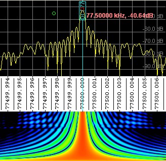
yet (use the "zero-pad" option in the FFT configuration dialog). The spectrogram
below shows the effect of
zero-padding :
The lower part of the spectrum shows a 'very broad' signal on 77.5 kHz, caused
by the zero padding. The upper part of the spectrum shows the *SAME SIGNAL*
(DCF77) after one hour of data acquisition, when about 14 percent of the
FFT input buffer was filled. It would have taken another six hours until
the full frequency resolution ( 40 uHz ) would have been reached.
Of course,
this level of FFT resolution can only be reached if the A/D converter's clock
frequency is sufficiently stable (the screenshot was made with an SDR-IQ
with a modified, temperature-stabilized clock oscillator, tied to DCF77 as
the frequency
reference).
Select the proper FFT window function for your application !
In most cases, the trusty old Hann window (named after Julius von Hann, not 'Hanning')
is a good compromise between frequency resolution (equivalent noise bandwidth = 1.5 times the FFT bin width)
and dynamic range (first sidelobes 32 dB below the main lobe, but rapidly decaying).
In other (extreme) cases, where dynamic range is more important than frequency resolution,
you may be better off with one of the 'new' flat-top windows.
For example, the same signal (a pure sinewave) analysed with Hann window, and one of the 'new flat-top' window functions:
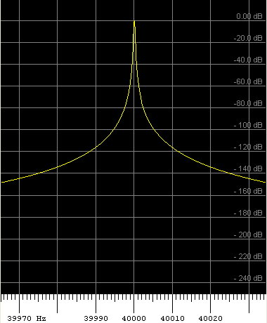

Left side: FFT with Hann window. Right side: Flat-top window with 196 dB sidelobe suppression (HFT196D by G. Heinzel).

Some of the FFT window functions implemented in Spectrum Lab,
plotted using DL4YHF's "CalcEd" (Complex Calculating Editor).
Since November 2003, the FFT is not only used in SpecLab's spectrum display, but also for a special audio filter which uses the FFT and the inverse FFT to realize very long FIR filters. How to use the FFT-based filters in SpecLab is explained here.
The IFFT (inverse FFT) which is mentioned in the description of the audio filter transforms a signal in the frequency domain (a "spectrum") back into the time domain. By principle, the IFFT is almost the same algorithm as the FFT - in fact, the FFT code is called as a subroutine from the IFFT code. If you are interested in this subject, follow the links to literature about digital signal processing (look for "The Scientist and Engineer's Guide to Digital Signal Processing", this book can hopefully still be downloaded for free in PDF format).
 25 coefficients, 2 bands,
 Band Lower Upper Value Weight
   1  0.000 0.120 1.000  001.0
   2  0.250 0.500 0.0001 100.0