IN3OTD's web site
...under perpetual construction.

Modeling a varactor capacitance vs. voltage curve
A while ago I started looking for a preselector circuit for an HF receiver; I was interested in controlling the preselector tuning using varactor, hoping to reduce the circuits size (maybe at the expense of performances, but that's another story...).
Realizing a filter that can be tuned over the entire 3 MHz to 30 MHz spectrum with using varactors is almost impossible, since that means covering a frequency ratio of 10 and so a capacitance variation of 100 over that frequency range; anyway to reduce the number of filters to be implemented it's better to select a varactor with a large capacitance variation with voltage
A good candidate is, for example, the MVAM125 tuning diode, which was designed for the tuning of AM receivers and has a specified capacitance ratio of 15 when changing the voltage applied from 25 to 1 .
Here is the capacitance vs. reverse voltage curve taken from the Motorola datasheet:
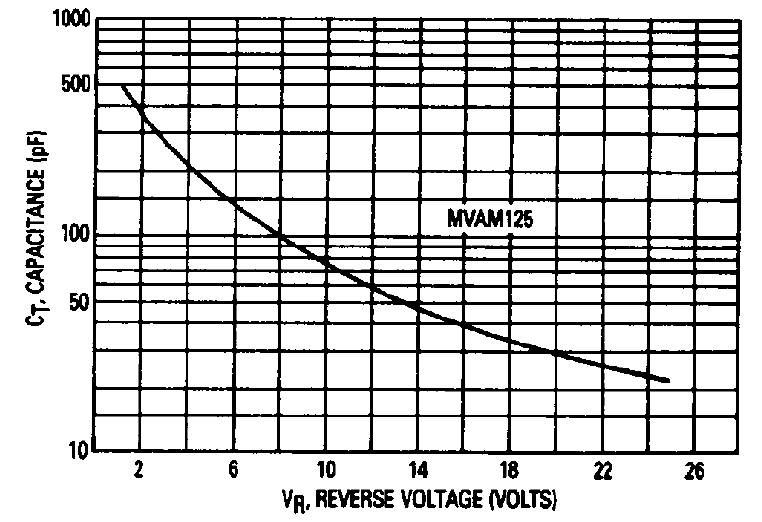
While having the C vs. V curve is essential, to be able to simulate the response of a circuit built using this component one needs to build a model for the circuit simulator. That means at first having the C cs. V data in a tabular form, instead of a graph, and then try to fit these data to an equation to model the capacitance variation with applied voltage
A very nice (and free, GNU GPL) application that can be used for extracting data from graphs is g3data; I have used it a few times in the past on graphs of different kind and quality and always obtained good results for the extracted data.
The following picture shows g3data at work on the MVAM125 capacitance curve shown previously:
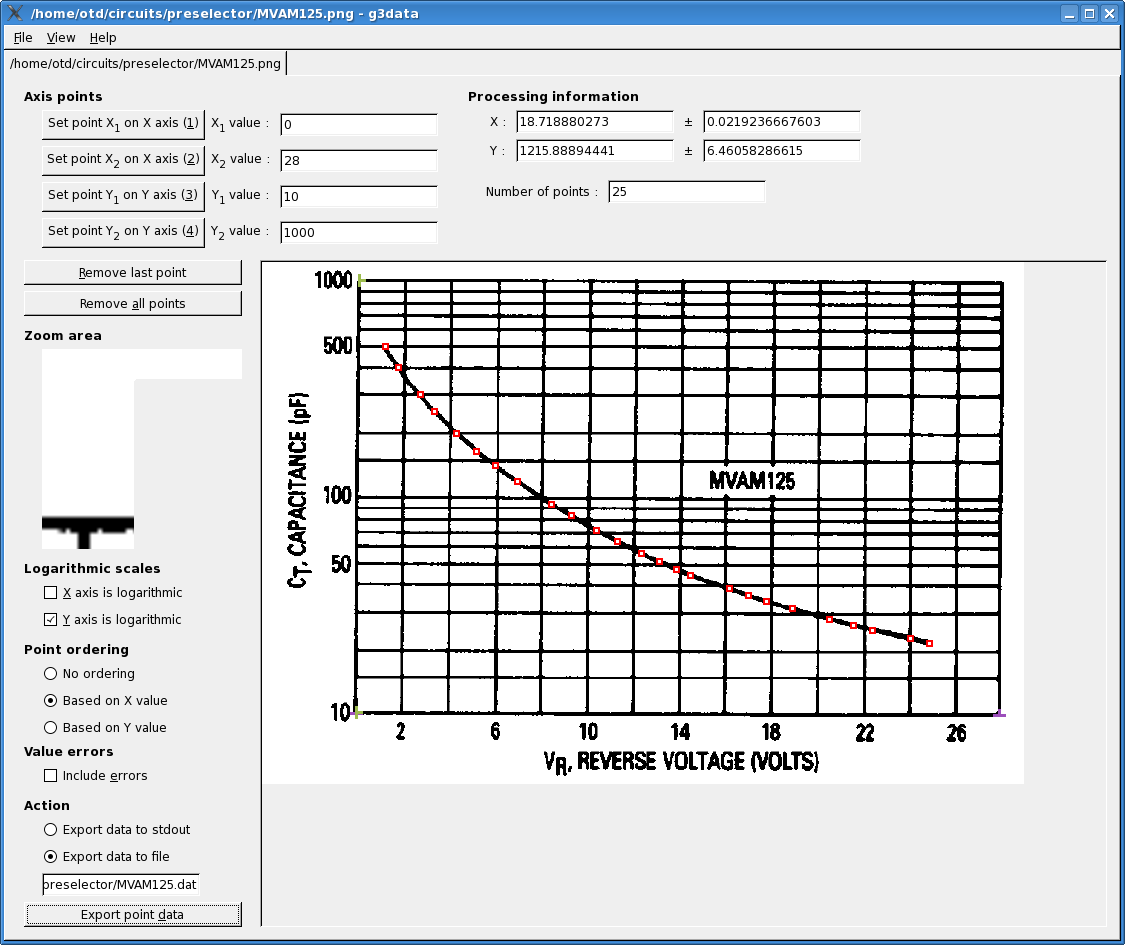 the end results of the data extraction process is a nice table with the coordinates of the selected points of the graph, expressed in voltage and capacitance:
1.15182409227  495.251088405
1.72425859127  396.088755583
2.69041190574  297.243255165
3.30518176124  248.091338324
4.26982309869  196.371630075
5.14616497829  162.194157989
5.97775233816  139.796207107
6.94057930319  117.961343317
8.42806229345  92.4166284689
9.30228740523  82.2457168559
10.3954467892  70.1504304649
11.3132168391  62.4320951781
12.3619240988  54.9792927709
13.1481521481  50.5152036284
13.8908352593  46.4120409989
14.5022787654  43.5567117967
16.2044624922  37.9693176637
17.0339330842  35.2614105339
17.8195563427  33.0964718297
18.9538415016  30.7432223568
20.5683305614  27.3752032402
21.6152234486  25.6995648082
22.4440892498  24.3810113593
24.1012160615  22.4162350293
24.9300818628  21.2661375771
Now that the C vs. V data are available in tabular for we need to fit a suitable curve; practically every circuit simulator has a model for the capacitance of a reverse biased junction which uses the standard equation [1]
C(v) = C0/((1+v/Vj)^m)
so this is the equation we will use for the data fitting.
There are several applications that can be used for curve fitting, a few specialized in this domain, other designed for general numerical analysis, like GNU Octave, but this time I have used the curve fitting capability of gnuplot.
I won't go into the details on how to setup gnuplot to fit a function to a set of data points, as this is well explained in the relevant section of the gnuplot manual.
Here is the gnuplot script that performs the curve fitting for our varactor capacitance:
c(x) = c0/((1+x/v0) ** m) 				# function to be fit
c0 = 1000; v0 = 0.5; m = 0.5;				# initial guess for c0, v0 and m
set fit logfile "mvamfit.log"
fit c(x) 'MVAM125.dat' using 1:2 via c0, v0, m

set key title "c(v) =  c0/((1 + v/v0) ^ m)\n"	        # title to key
set title "MVAM125 capacitance and curve fit"
set pointsize 1.5 					# larger point
set xlabel 'Voltage [V]'
set ylabel 'Capacitance [pF]'
set xrange [0:26]
set yrange [10:1000]
set ytics (10,20,50,100,200,500,1000)
set logscale y
set grid

plot 'MVAM125.dat' using 1:2 title 'Datasheet' with points 3, \
      c(x) title sprintf('Curve-fit; c0 = %f, v0 = %f, m = %f', c0, v0, m)

set term push						# save current terminal settings
# write the graph in PNG format
set terminal png
set output "MVAM125_Cfit.png"
replot;
set term pop						# restore saved terminal settings


# show error in curve fit
set title "MVAM125 curve fit error"
set key left top default
set ylabel 'error [%]'
set yrange [-5:5]
set ytics autofreq
unset logscale y
plot 'MVAM125.dat' using 1:(100 * (1 - c($1)/$2)) with linesp

set term push						# save current terminal settings
# write the graph in PNG format
set terminal png
set output "MVAM125_Cfit_error.png"
replot;

set term pop						# restore saved terminal settings
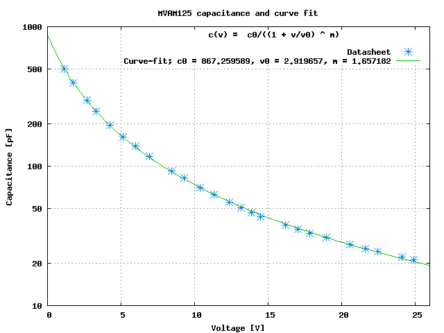
and here is a graph which shows the data point extracted from the datasheet curve with the function fitted by gnuplot:
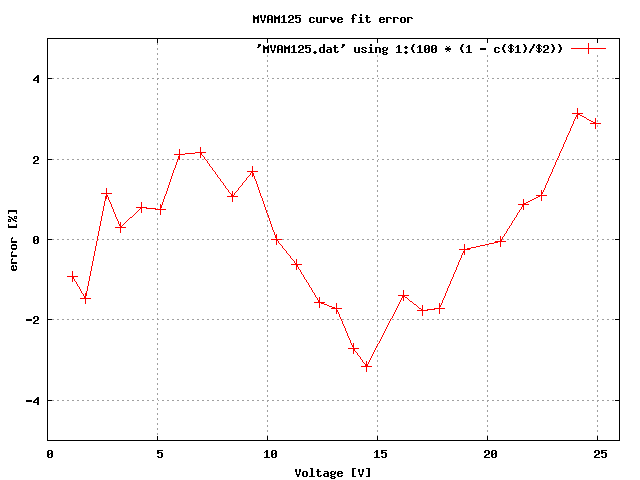
 results seems not too bad; to better evaluate the curve fit quality here is a graph of the errors between the data points provided and the fitted curve:
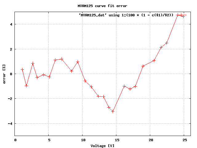 From this latter graph it's evident that the fitted curve error increases for the points corresponding to a higher voltage and lower capacitance. This is due to the way the curve fit is done: since the curve fit algorithm tries to minimize the sum of the errors squared, the points with a lower value will have a higher relative error.
To have a better fit also on the low-capacitance side we can tell gnuplot to weight the errors according to the data points value with a simple modification to the script. These are the results of this weighted curve fitting:
 the error in the data fitting has improved, so now the low-capacitance points have a little less error, at the expense of the higher-capacitance points:
So, in the end, the capacitance of our MVAM125 varactor diode can be modeled by the equation
C(v) = 867.3/((1+v/2.9)^1.66) [pF], v in Volt
of course other important aspects of the model, like the series or parallel resistance have not been taken into account, but can be always introduced in the model later, if needed.
References:
| [1] | G. Massobrio and P. Antognetti, "Semiconductor Device Modeling with SPICE," McGraw-Hill, 1st ed., Dec. 1998. |