Special features for the Earth-Venus-Earth
experiment
Author: Wolfgang Büscher, DL4YHF .
Thanks to Karl Meinzer (DJ4ZC), Achim Vollhard (DH2VA), Hartmut Paesler (DL1YDD),
Freddy de Guchteneire (ON6UG), James R. Miller (G3RUH), and Markus Vester
(DF6NM) for their explanations; and to everyone else at AMSAT-DL in Marburg
and at the IUZ in Bochum for the opportunity to take part in this experiment.
Updated 2009-03-27 : AMSAT-DL successfully received
their own echoes from Venus on 2.4 GHz at the radio telescope in Bochum
!
Contents
-
Introduction
-
Setting up SpecLab for the experiment
-
Synchronisation of receive / transmit periods
-
Theory of operation
-
Theoretic ratio of signal-plus-noise to noise
(SNNR)
-
Standard deviation in the average spectrum versus
SNNR
-
Generation of a "test signal"
-
Analysing I/Q wave files (recorded with
SpectraVue)
-
Real-time signal analysis with
SDR-IQ and Spectrum Lab
-
The noiseblanker (added for the AMSAT EVE
Experiment)
-
RX/TX control (inside the Spectrum Lab
application)
-
Control buttons (on the left side of the main window)
The Earth-Venus-Earth experiment (EVE) by AMSAT-DL in Bochum finally succeeded
!
Details are on the
AMSAT-DL
website, and in the AMSAT-DL journal (July 2009).
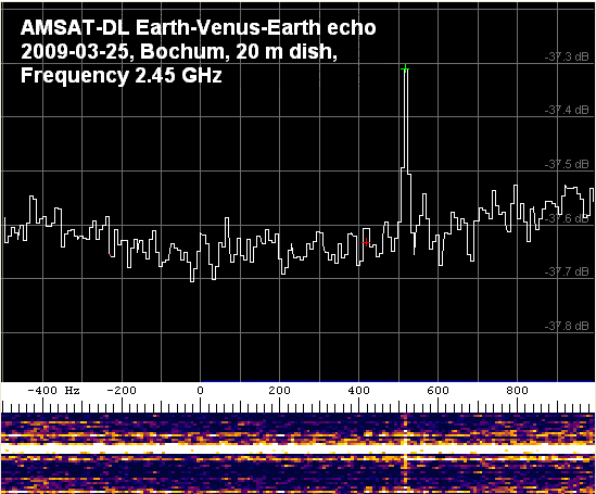
Screenshot of a long-term average power spectrum; integration time about
50 minutes.
The fuzzy horizontal line in the spectrogram is caused by kitchen magnetron
QRM.
The thin vertical line near 500 Hz ("audio") shows the Venus reflection .
Displayed timescale is 50 minutes.
Bochum, March 25th, 2009 .
Spectrogram showing AMSAT-DL's "HI" message in very slow morse code (....
..), bounced off Venus.
The entire transmission / reception of this morse code took almost two
hours.
Bochum, March 26th, 2009 .
Brief description of the EVE experiment :
-
20 meter parabolic dish antenna (Bochum IUZ) with Cassegrain subreflector,
-
Antenna 3 dB beamwidth measured to be 0.42 degree
-
a team of 9 highly motivated radio amateurs to operate, and many more to
build the system described below...
-
a 6 kW magnetron transmitter, tamed for CW (and SSB!) operation, locked to
a Rubidium frequency reference (which was checked against a GPSDO)
-
mechanical coarse tuning of the magnetron using a slider in the output waveguide,
controlled with a DC servo motor
-
Magnetron control unit by Karl Meinzer using 2 * 4CX1000 as current regulators
in a loop with over one MHz bandwidth,
making it possible to produce SSB signals with the magnetron (which, without
Karl's circuit, would be an unstable free running power oscillator).
Anode voltage about 7 kV, anode current about 1.2 A, fast frequency control
via anode current (through the 4CX1000).
-
Magnetron remotely controlled and supervised via microcontroller, connected
to an extra PC via serial port, visualisation (by DH2VA) on an extra PC running
LabView
-
Precise azimuth- and elevation control, accurate antenna tracking system
and permanent Doppler frequency compensation (all controlled by software
from G3RUH)
-
low-noise amplifiers, downconverter from 2.4 GHz to ~190 MHz to avoid the
cable loss between antenna and control room on 2.4 GHz
-
system noise temperature estimated 93 K, measured about 85 K
-
AOR AR5000 receiver with CAT control (for the Doppler compensation) and 10.7
MHz IF output
-
lots of other important stuff I forgot to mention (please bear with me..
Karl, Achim, Freddy, Hartmut, Hermann, James, Max, and all)
-
5 minute transmit- followed by 5-(or 10-) minute receive intervals while
Venus was 42.1 million kilometers away from Earth
-
Software Defined Radio with digitized output (I/Q) via USB to feed the 10.7
MHz IF signal into the PC.
Note: The SDR's sampling clock was not tied to the AMSAT's 10-MHz Rubidium
frequency reference during this experiment yet !
-
FFT software (SpecLab), operated by its author ;o) for the comparably trivial
task to dig the weak signal out of the noise
-
noiseblanker implemented in software to defeat WLAN QRM
-
8138 samples per second, 1024 point FFT with Hann window, 50 percent overlap
(between blocks in the time domain), giving an FFT frequency bin width of
7.9 Hz and an equivalent receiver bandwidth of 11.9 Hz (due to the FFT
windowing). Using a rectangular window didn't change the observed SNNR
(signal-plus-noise to noise ratio) too much.
The Venus reflections were 8 to 11 dB below the noise in a 10 Hz equivalent
receiver bandwidth, and showed up on the screen as a "peak" with 0.3
to 0.4 dB SNNR. The limiting factor was not the receiver's system noise
temperature (which was excellent thanks to the work of the AMSAT crew in
Marburg and Bochum), but the annoying "woodpecker" noise cause by wireless
LAN in the 2.45 MHz ISM band. This frequency had to be used because of the
magnetron tube's resonant frequency, and the limited tuning range of 10 MHz
(maximum). Plans are under way to find a magnetron for a slightly lower
frequency. (BTW if you have one or two 6 kW magnetron tubes operating on
2400 MHz or a bit lower, and would donate or sell it for a fair price, please
contact Karl Meinzer DJ4ZC at AMSAT-DL).
The only way to defeat the WLAN-QRM was a special noiseblanker with *constant*
(but parametrizeable) threshold level. That blanker can be activated in the
first "DSP blackbox". Since the SDR-IQ was used, the noiseblanker must process
the inphase ("I") component, and the quadrature ("Q") component at the same
time (in contrast of the older noiseblankers). The parameters of this "AMSAT
EVE Noiseblanker" can be modified in the test circuit (right-click on the
DSP blackbox to see it). During the experiment in March 2009, the parameters
were:
- pre-trigger 0.5 ms (which means 0.5 milliseconds BEFORE the noise burst
is detected will be blanked)
- post-trigger 0.5 ms (which means 0.5 milliseconds AFTER the noise burst
is detected will be blanked)
- trigger level 12000 (on a scale ranging from 0 to 32767 "ADC units")
During most of the time, only a few "woodpeckers" (WLAN beacons) exceeded
the noiseblanker threshold, so only 3 to 10 percent of the received signal
got lost. A hard limiter may also work effectively, but this was not tested
yet.
One day after the first successful "contact", the AMSAT crew successfully
sent a "HI" message in very slow morse code to Venus, and received the echo.
But this took more than 20 times 5 minutes (go figure..). The raw signal,
received with an SDR-IQ, was saved in chunks of 5 minute intervals, 16 bit
per sample, 8138 samples/second, "stereo" because the samples are
complex). The following files may be available on the AMSAT-DL website
(caution, they are about 9 MByte per file) :
EVE-090326_094053.wav (i.e. recording started 2009-03-26 09:40:53,
which is the first 5-minute-block)
to
EVE-090326_112556.wav (i.e. recording started 2009-03-26 11:25:56,
which is the last 5-minute-block)
If you listen to these files with an normal audio player, you'll only hear
periodic woodpecker-like signals, and occasional strong buzzing or hissing
noises. The latter are -most likely- kitchen magnetrons operating in the
2.4 GHz ISM frequency range. The procedure to make the "HI" slow morse
code visible in these recordings will be described later (either here,
or in the AMSAT journal, or on the next AMSAT-DL meeting).
Introduction (about the signal processing for the EVE
experiment)
In 2007, some new features were implemented in Spectrum Lab for an experiment
with the 20-meter parabolic dish antenna at the
IUZ in Bochum. The principle
(refined in 2009, when the operating frequency was changed from 10 GHz to
2.4 GHz) :
-
Transmit a microwave signal towards Venus for 5 minutes. Estimated
parameters:
Antenna gain = 63.5 dBi, transmitter output power = 600 W (on 10 GHz),
EIRP = 600 W * 10^(63.5/10) = 1.34 GW . (on 10 GHz; less antenna gain but
more TX power on 2.4 GHz)
-
Switch from transmit to receive, and wait for the (theoretic) arrival of
the signal. Parameters:
noise temperature = 120 K, antenna gain = same as on transmit .
-
Receive for 5 minutes, analyzing the 10 GHz signal with an equivalent receiver
bandwidth of 40 Hz (or so), and add all FFTs within this period to reduce
the noise (and increase the signal-to-noise ratio).
For 2.4 GHz, the RX bandwidth will be approximately 10 Hz to match the expected
reflections.
-
Plot a single line on the waterfall screen (spectrogram), representing the
spectrum of the 5-minute reception cycle,
-
repeat the above steps over and over, until a sufficient number of FFTs is
captured.
In addition to the above, the average of ALL lines in the spectrogram buffer
(= ALL FFTs since the start of the experiment) is calculated, and displayed
as a curve in the spectrum graph window. This should result in an additional
noise reduction (or, more precisely, flattening of the noise floor in the
spectrum), so we hope (!) that, after a sufficient integration time, the
reflected signal will become detectable in the long-term spectrum graph.
The expectable signal-to-noise ratio -under optimum conditions- is explained
in a later chapter.
There are, of course, a few obstacles :
-
The reflected signal will be appear "smeared" (or broadened in the frequency
domain), partially caused by the sulphur acid atmosphere on Venus - which
is everything but an ideal reflector for radio waves. The reflected 10 GHz
signal is expected to be 40 .. 100 Hz wide, so an effective receiver bandwidth
( ~ FFT frequency resolution aka "bin width") of 40 Hz or a bit less
sounds appropriate. The spreading of the reflected signal will depend on
where the signal is reflected - the Venus atmosphere will produce more doppler
spreading than reflections on the ground.
-
The SNR on 10 GHz will be very low, in the range of -20..-22 dB S/N in a
40 Hz RX bandwidth (some uncertainty, because the exact reflectivity of Venus
on 10 GHz is unknown).
-
The SNR on 2.4 GHz will be a bit better; some preliminary estimations by
DJ4ZC:
The reflected signal is expected to be about 10 Hz wide; 7 to 8 dB below
the noise level (thanks to the considerably larger TX output on 2.4 GHz);
so with some luck the reflection should be detectable after a few 5-minute
periods already (more on that after March 2009, hopefully...)
-
There is some passband ripple in the RX system, which may change during the
3 hour integration time. Only the passband ripple caused by the DSP filter
(in the software defined radio) can be eliminated or compensated.
The following chapter describes how Spectrum Lab was used for the Bochum
experiments. Please note that some of the details have already been superseded
- for example the soundcard is not used anymore-, but the principle explained
in the next chapters remains unchanged.
There will be a special configuration file in the CONFIGURATIONS directory,
called EVE-IQ-44kHz.usr (for the soundcard sampling at 44.1 kHz). To analyze
I/Q samples directly received with SDR-IQ, or audio files saved with SDR-IQ
/ SpectraVue, use EVE-IQ-5kHz.usr instead.
There is also a fast-running "simulator" for this experiment
(EVE_Simulator.usr ). It uses a synthetic test signal instead of the microwave
receiver which will be used in the experiment later. While the simulator
runs, look at the red line in the spectrum graph - it is the
long-term average
spectrum, which should (if all works as planned) slowly creep out of
the noise, as more and more signal energy is accumulated. Details about the
theory, and the test signal generator settings follow in the chapter
Generation of a Test Signal.
To load one of these files, use
"File".."Load Settings" in the main menu. Alternatively, you can add this
configuration to the "Quick Settings" menu ("Quick Settings"..."Load and
Create User Defined Entries"). This allows you to switch quickly between
different configurations. All configurations for the Earth-Venus-Earth experiment
begin with the prefix "EVE_" .
If you want to modify the configuration, or write your own configuration
instead of using one of the preconfigured "EVE"-settings, here are the necessary
steps:
-
Set the display in the main window to combined display mode (which means,
the spectrum graph in the upper part, and the waterfall (spectrogram) in
the lower part of the window: Right-click into the waterfall or spectrum
graph area to open a context menu, and turn on "Waterfall" and "Spectrum
Graph" if not already active.
-
Turn on the "Long-term Average Graph" in the Spectrum Graph window:
Right-click into the Spectrum Graph area to open a context menu, point at
"Long term average spectrum", and click on "show Long-term average graph"
if not already checked (there is a checkmark near this menu item, which is
set if the option is already active). On this occasion, you can also turn
on the Auto Range function (in the same menu under "Spectrum Graph Options".
This will automatically switch the amplitude scale in the spectrum graph
for best visibility, which helps a lot as the long-term integration proceeds.
-
Select a suitable sampling rate for the soundcard, at least two times the
maximum audio frequency of the radio. For a typical "SSB" receiver, 11 kHz
is sufficient. If you plan to record the "raw audio" while the experiment
is running, don't make the sampling rate larger than required because you
may get increadibly large wave files ;-). How to:
In the main menu, select "Options"..."Audio Settings"..."Sample Rate
(nominal)".
(ToDo: Modify this step as soon as the SDR-IQ downconverter is directly
supported)
-
Select a suitable FFT size, which results in an effective receiver bandwidth
of 10...100 Hz (see considerations above; we may want to tell "stable carriers"
from "Venus reflections" by looking at the spectrum a bit closer). Example:
11 kHz sampling rate, 1024-point FFT -> Width of one FFT-bin = 10.7 Hz,
Equivalent noise bandwidth = 16.15 Hz (due to the Hann FFT window). The FFT
settings can be accessed through the main menu, select "Options"..."FFT
Settings".
-
Check the "Display Settings, part 1":
Set the option "Optimum Waterfall Average". This causes SpecLab to calculate
a new FFT every few hundred milliseconds, which will be added to the first
averaging stage. The internal FFT calculation interval is automatically set
for a 50 percent overlap between to FFTs (if an FFT windowing function other
than the "rectangle" window is used). For example, at 11 kHz sample rate,
and an FFT length of 1024 points, a new FFT will be calculated every 0.5
* 1024 / 11025 Hz = 46 ms. The "momentary" FFTs will be frequently shown
as a blue curve in the Spectrum Graph window (more precisely, this curve
is drawn with "Pen number 2", if you have modified the colours...). More
info about spectrum averaging can be found
here (in the SpecLab
help system).
-
Next, set the Waterfall Scroll Interval to 30 seconds. This will produce
about 10 lines in the waterfall during the 5-minute reception period, which
allows us to quickly spot "problems" in the waterfall. This setting does
not affect the SNR of the finally calculated spectrum (long term average),
because the final result is the average of ALL calculated FFT's.
During an initial test in Bochum, it turned out that the soundcard wasn't
up to the job as explained later . The
soundcard was replaced with a digital downconverter called SDR-IQ (details
in one of the next chapters).
There are different possible ways to achieve synchronisation:
-
The most simple solution (from SL's point of view) is to simply let the waterfall
run all the time, also during the TX-overs. This is possible if the receiver's
audio output is "muted" during transmission, or -at least- there is no signal
near the expected Venus reflection.
-
Alternatively, one could use SpecLab itself to produce the 5-minute-RX/TX
cycles, using the serial port as the PTT switch ("push-to-talk", actually
the RX / TX switch of the HF radio), and/or an audio tone to modulate the
transmitter, generated with the test signal generator (and fed to the output).
The "periodic actions" or "conditional actions" can be used to switch the
PTT, and turn the audio tone on and off. (ToDo: more on this if required).
The waterfall can be paused during the TX-periods, using the interpreter
command "sp.pause=1" (pauses the frequency analyser and the waterfall) and
"sp.pause=0" (resumes normal operation, "not paused").
To make things even simpler, the waterfall can be paused and resumed via
programmable button with hotkey. There is an example for this in the first
"test" configuration, using the programmable buttons in the main window (labelled
"Pause" and "Continue").
-
The third method uses an input signal on the serial port to control the spectrum
analyser. The external control signal can be fed to the PC's serial port,
and used in one of the "Conditional Actions" to start and stop the calculation
of FFTs.
This is the method actually used in the tests at the IUZ in 2007-07-27, details
in a later chapter .
As explained in the introduction, the expected SNR (signal-to-noise ratio)
will be very low; for example -21.6 dB (*) in
a 40 Hz (**) bandwidth. But how can
such a weak signal be made visible, especially since it is incoherent, "40-Hz
wide or more" ?
-
(*) estimated by DJ4ZC for
an albedo of 1 percent (albedo = measure of diffuse reflectivity) on 10
GHz.
The figures for 2.4 GHz look more promising..
(**) 40 Hz is the expected bandwidth
if most of the 10 GHz signal is reflected on the surface.
For the test on 2.4 GHz, replace the 40 Hz by
10 Hz (equivalent receiver bandwidth).
The FFT splits the signal into a number of "frequency bins". The spectrum
graph or spectrogram is more or less a graphic representation of the FFT.
In the case of the EVE signal, it shows mainly noise; just a few frequency
bins additionally contain the weak signal reflected from Venus. We cannot
read the SNR directly off the screen, only the SNNR (signal-plus-noise to
noise ratio - details in the next chapter).
Longer FFTs to get additional gain (gc/dB = 10*log10 of
the bandwidth ratio) don't help here, because the reflected signal
is not coherent (it is possible to use a longer FFT, but in that case the
"FFT Smoothing" option must
be turned on to match the overall filter to the signal). A 40-Hz receiver
bandwidth matches the expected signal bandwidth for the 10 GHz test. The
only chance is integrating the signal energies (in the FFTs) over a long
time, to reduce the standard deviation in the "long term average spectrum"
(which is the red graph displayed in SpecLab). Increasing the integration
time (or "number of FFTs") reduces the standard deviation
(sigma) by the square root of the number of FFTs.
-
This "gain" (gi, gain from incoherent integration) can be
calculated in decibel as :
-
gi/dB = 10 * log10 ( sqrt( number_of:_FFTs ) )
-
Example: 1 million FFTs :
-
gi = 10 * log10 ( sqrt( 1000000 ) ) dB = 30 dB .
With the FFT window set to "Rectangular" in SpecLab, there is no overlap
between the FFTs, and collecting data for an FFT with 40 Hz bin width takes
25 milliseconds.
-
Note: A soundcard running at 11025 samples/second, and a 256-point "real"
FFT, give a 43 Hz FFT bin width, and 23 milliseconds time to acquire the
samples for every FFT. The output of the simulation after three hours of
integration is shown here . If
the SDR-IQ is used (with 8138 samples/second), each of the 256 FFT bins will
be 32 Hz wide, but the principle remains the same.
Aquiring the data for 500000 FFTs (gi=28.5 dB) with 40 Hz FFT bin width requires
3.5 hours, and 300000 FFTs (gi=27.4 dB) 2 hours of signal integration. This
doesn't take the 50 percent RX/TX duty cycle into account yet !
In the previous chapter we saw that the signal is 'way down in the noise',
even in the equivalent receiver bandwidth. In other words, the FFT gain isn't
enough to lift the signal above the noise. For example, the 10 GHz reflection
may be 21 dB below the noise in a 40 Hz receiver bandwidth. On 2.4
GHz, the signal was 8 to 11 dB below the noise in a 10 Hz receiver bandwidth,
depending on the weather conditions, and the ISM noise despite the noiseblanker.
The long-term average spectrum shows the averaged signal energies (on a
logarithmic scale), using 40 (or 10) Hz wide "frequency bins". Ideally, with
white gaussian noise on the input, all bins will filled to the same average
level after an infinite time (when sigma reaches zero).
Ideally, only one of the frequency bins contains additional energy from the
Venus reflection. For an SNR (signal to noise ratio) of -21.6 dB, the
Signal-plus-Noise to Noise Ratio would be :
SNNR = 10 * log10( ( 1 + 10^( SNR / 10) ) ) = 10 * log10( ( 1 + 10^(-21.6
/ 10) ) ) = 0.0299424 (dB) .
-
where
-
SNNR = Signal-Plus-Noise to Noise Ratio in dB
SNR = Signal to Noise Ratio in dB,
log10(x) = ten's logarithm of x,
10 ^ x = ten power x .
-
So, after an infinite time of integration (i.e. sigma dropped to almost zero),
the "21 dB below the noise signal" will appear as a 0.03 dB "peak" above
the noise level.
Of course we cannot wait for an infinite time (until the noise in the spectrum
graph is "sufficiently flat"). How long must this signal be integrated, until
it becomes visible in the spectrum graph ? See next chapter !
Without an infinite time of integration, the sigma value (in the averaged
powers, or energies, in all FFT bins within the observed frequency band)
will not drop to zero, but to:
sigma(dB) = 4.34 / sqrt(n) ,
-
where
-
sqrt(n) = square root of n,
n = number of integrations (number of the power FFTs, added in the long-term
average)
For example, with 50000 averages from a white noise signal, the resulting
standard deviation in the frequency series (average FFT) would be
sigma = 4.32 dB / sqrt(500000) = 0.0061094 dB .
Note: The measured "sigma" value is displayed on one of the
programmable buttons during the experiment, along
with the average counter. The sigma value should be monitored occasionally.
If it doesn't decrease as the average counter increases, watch for manmade
noise !
The table below shows some theoretic, and a few measured sigma values.
| Number of averages |
1 |
2 |
10 |
100 |
1000 |
5000 |
10000 |
50000 |
100000 |
500000 |
| Theoretic sigma (1) |
4.32 dB |
3.05 dB |
1.36 dB |
0.42 dB |
0.14 dB |
0.061 dB |
0.043 dB |
0.019 dB |
0.014 dB |
0.0061 dB |
| Measured sigma (2) |
|
|
|
0.41 dB |
0.15 dB |
|
0.041 dB |
0.023 dB |
|
|
(1) Sigma values calculated
with DL4YHF's
CalcEd, using
the file eve_calc.txt (plain ASCII). Values rounded
to two decimal places.
(2) Sigma measured with
a Perseus (SDR) running at 125 kSamples/second, VFO set to 10.7 MHz,
fed with noise only, ripple compensation enabled, 16384-point FFT, Hann-window,
measured between 300 and 1500 Hz (baseband) using the interpreter expression
"sigma(#LTA1,300,1500)" .
To identify the signal in the averaged power spectrum, we want the SNNR to
be 4 times stronger than sigma. In other words, if the signal-plus-noise
to noise ratio is four times larger than the standard deviation in the frequency
bins, we can be sure enough that we're not looking at a random peak (see
screenshot in one of the next chapters).
Example (with the assumed parameters for the 10 GHz test):
SNNR = 0.03 dB (approx., theoretical)
-> sigma must drop below 0.03 dB / 4 = 0.0075 dB .
Under ideal conditions (i.e. perfect passband ripple compensation, and only
white noise added to the Venus signal), this sigma is reached after
N_Averages = (4.32 / Sigma)^2 = (4.32 / 0.0075 dB)^2 = 333000 .
Collecting data for this number of averages (for an FFT with 40 Hz bin
width) takes about
333000 / 40Hz = 8326 seconds, or 2.3 hours .
If we decide we can see the signal when sigma has dropped to SNNR
/ 3 (instead of SNNR / 4), the integration time drops from 2.3 to 1.3
hours.
For the 2.4 GHz experiment, the figures looked more promising (see the
update from March 2009 with an actual screenshot
showing the Venus reflections): Expected SNR about -8 dB in a 10 Hz receiver
bandwidth, eventually a bit less due to the ISM / WLAN / kitchen magnetron
noise.
To check the proper function of the long-term spectrum average, a sufficiently
"weak" test signal was created using SL's built-in test signal generator.
The following values apply to the 10 GHz experiment (divide the bandwidth
by 4 for the 2.4 GHz settings). The output "amplitude" of the noise generator
in SL was set to -50 dB / sqrt(Hz), and one of the sine wave outputs to -55
dB (Note: all these dB-values are relative to "full scale"; 0 dB is the clipping
point of the soundcard).
-50 dB noise in a 1 Hz bandwidth is equivalent to (-50 +
10*log10(40Hz/1Hz) ) dB = (-50 + 16) dB = - 34 dB noise power
in a 40 Hz bandwidth; so the sine wave is (55-34=) 21 dB "below the noise"
in a 40 Hz receiver bandwidth. So far, so good... but how does it work in
practise ? The following diagram shows the resulting spectrum
after three hours of averaging:
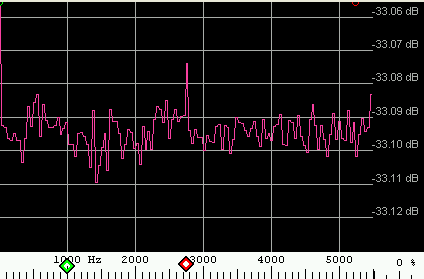
The red diamond marks the frequency of the sine wave generator (in the simulator
configuration).
Note: The "real" noise from the receiver will not look as good ("flat") as
this one.. there will be some passband ripple which is not considered in
this simulation !
In older SpecLab versions, the SDR-IQ downconverter was not directly supported
by Spectrum Lab. So the 5-minute receive periods had to be saved as stereo
wave files (*); so they can be
post-processed with Spectrum Lab. How to do that ....
-
Load the configuration "EVE-SDR-IQ-5kHz" as explained in a previous chapter
(for simplicity, add this configuration to one of the entries in the "Quick
Settings"-menu).
-
Stop the "Sound Thread" (in the main menu: Start/Stop) if the audio processing
still runs in real time (using input from the soundcard, or the SDR-IQ
converter).
-
Clear the "Long Term Average Spectrum": right-click into the spectrum graph
area, and select "Long-ter m average spectrum"..."Clear.." in the popup menu.
This is important, otherwise you may be fooled by old data in the average
buffers !
-
Select all recorded files (or the "next recorded" file) for analysis:
In the "File" menu, select "Analyse Audio File (without DSP)". There is an
important trick how to select multiple files in a windows file selector
box:
- Click on the first file, then press and hold the SHIFT key ("Umschalttaste"),
and select the last file .
OR :
- Select multiple individual files while holding the CONTROL key ("Strg").
Click "OK" in the file selector box when ready.
-
A special dialog titled "File Analysis" is displayed, which shows some parameters
of the first analysed wave file. Make sure the option "play/analyse this
file in an endless loop" is not set. Then click "OK".
-
The program will analyse the wave file now, much faster than it was recorded
(that's the difference between the functions "Analyse File (without DSP)"
and "Analyse and play file (with DSP)" ).
-
When the new file (or all files) has been analysed, the analysis stops.
You can select a new file now (as soon as SpectraVue has recorded a new one),
or try the entire analysis again with modified parameters (different FFT
size, with or without automatic gain control, with or without passband ripple
equalisation, etc etc).
-
(*) Why use SDR-IQ,
and not the soundcard ?
-
During a test in Bochum, we found that there were a lot of "spikes"
in the 10 kHz region, caused by the frequency converter which drives the
azimuth / elevation rotors. A typical EMC problem... which seriously affected
the signal entering the soundcard. The SDR-IQ (an interesting and affordable
software defined receiver / downconverter by RFSPACE) did not suffer from
this problem, because it directly processes the 10.7 MHz IF and sends it
via USB to the PC. So we decided to use it instead of the soundcard). At
that time, we used the SpectraVue software to record the SDR-IQ's output
in blocks of 5 minutes, with 37 kHz sampling rate.
In the meantime, Spectrum Lab directly supports SDR-IQ so the data can be
analysed in real time. Also, the 5 kHz audio bandwidth (8.1 kHz sampling
rate) can be used, which greatly reduces the size of the recorded audio files,
and the CPU time required to analyse the data. Furthermore, the passband
ripple can be compensated using a file provided by RFSpace - see
passband ripple compensation in the next
chapter.
After analysing 3 hours of samples, or about
340000 256-point FFTs with 32 Hz bin width, the long-term average spectrum
looked as shown below. Data were collected with SDR-IQ running at 8138 Hz
sampling rate, fed with "real noise" from the microwave transverter. Only
the Venus-signal was "simulated" with a stable RF generator; 21.6 dB below
the noise in a 32-Hz FFT bin.
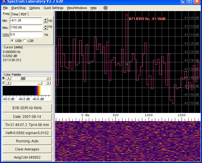
The red curve in this diagram is the long-term average. The readout cursors
(red and green cross in the graph) mark the generator signal. The difference
between (signal+noise) and noise in an FFT frequency bin (32 Hz) is 0.03
dB after three hours of integration. The standard deviation (sigma, here
indicated as 0.0102 dB) is slightly higher than the theoretic value; but
this is caused by the remaining passband ripple (which could be reduced further
by using an improved compensation table). The ratio between signal-plus-noise
to noise (i.e. the 0.03 dB mentioned above) comes close to the theoretic
value calculated here. But remember, the
noise was real, but the "Venus" signal was in fact Hartmut's RF generator
;-)
To reduce the CPU load, the passband ripple, and the file size, we will let
the SDR-IQ run at f_sample = 8.1 kHz (which results in an observed bandwidth
of 5 kHz). The optimum parameters were unknown at the time of this writing,
so just a few short notes:
-
The preferred configuration (as of 2007-08) is EVE-SDR-IQ-5kHz.USR . Load
it as explained earlier.
-
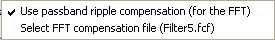
Passband ripple compensation: For a passband ripple
below 0.01 dB, the EVE-configuration loads the correct "FFT compensation
file". These files are part of SpectraVue (the software which comes with
the SDR-IQ radio, by RFSPACE; usually these files are located in
c:\Programme\SpectraVue\FilterComp). For the 5 kHz bandwidth setting,
"Filter5.fcf" is used. If you need to create your own configuration: From
SpecLab's main menu, select "Options".."SDR-IQ / SDR-14 Settings". Then,
in the SDR-IQ control panel, on the "CFG"-tab, click on "More...".."Select
FFT Compensation File". Then find your way to the SpectraVue/FilterComp
directory, and select "Filter5.fcf" (or the file designed for the sampling
rate you use). After that, turn on the compensation in the menu "Use passband
ripple compensation". When the option is active, there's a CHECKMARK before
the menu text:
-
In this configuration, one of the programmable buttons shows the number of
averages collected the start of an experiment. The long-term average (which
is the most important result) can be cleared with the button "Clear Averages".
Click this button only once before starting a new 3-hour integration (if
you click it by accident, don't worry; you can do a new average calculation
off-line, using the recorded 5-minute wave files with the raw baseband
data.
Details about the programmable buttons in the EVE-configuration are
here .
-
The automatic RX/TX switching starts the analyser 1 second after the begin
of a receive period, and stops the analyser 1 second before the end of a
receive period. Together with the spectrum analyser, the recording of I/Q
baseband data is also started and stopped automatically. For details about
RX/TX Control (as used in Bochum), see next chapter.
-
In addition to the automatic RX/TX switching, the analyser can also be started
manually by clicking on the button labelled "Paused, Auto". Details are also
in the next chapter.
-
If there is a problem with the SDR-IQ, or you need to disconnect it from
the USB port, first STOP the real-time processing ! While the yellow LED
on the SDR-IQ is flashing rapidly, it sends I/Q data. DO NOT DISCONNECT the
USB cable in that case. To stop it, select "Start/Stop" ... "Stop Sound Thread"
in SL's main menu. To start it again, select "Start Sound Thread" in the
same menu.
-
If the USB communication between SDR-IQ and PC breaks down for some reason:
The program usually detects this automatically and restarts the communication
immediately (so you don't have to do anything). Only in the rare event that
USB communication "breaks down completely" (*), stop and restart the sound
thread as described in the previous paragraph.
-
(*) Why should the USB communication "break down", and how to notice that
?
-
The reason may be a severe, but temporarily overload of the analysing PC.
If that happens, the SDR-IQ stops flashing its yellow LED rapidly, and the
"input"-block in SL's circuit window
turns red instead of green.
The SDR-IQ seems to monitor if data from the USB arrives periodically (not
sure how yet, but there seems to be a watchdog-like "timeout monitor" in
it).
Spectrum Lab alsoy monitors if data from the USB port arrive in regular
intervals. If that doesn't work, it tries to establish communication again
by sending a special command to the radio. If that fails, too, the "input-block"
in SL's circuit window turns red instead of green. BTW, the colours in the
circuit have the following meaning:
GREEN=active/ok; YELLOW=busy/waiting/being configured; RED=error;
GRAY=passive.
Even with the 20 meter dish antenna used in the March 2009 EVE experiment,
noise from a nearby WLAN (operating near 2.45 GHz) could not be reduced to
a sufficiently low level. The power spectrum was dominated by some
woodpecker-like sound ("tack-tack-tack"), so a noiseblanker was implemented
in software to get rid of this noise. It is inserted in the signal processing
chain before the FFT.
To analyse (and record!) only the receive-phases during the experiment, one
of the input signal on the RS-232 interface is used to sense the current
RX- / TX state of the equipment. Inside the Spectrum Lab application, the
programmable 'conditional actions' are used for that purpose. They permanently
work "in the background" to control the following:
-
While the radio transmitter is ON, the spectrum analyser is stopped, and
no data is recorded to a wave file
-
On the transition from TRANSMIT to RECEIVE, the analyser is started, and
a new wave file (with the current date+time in the filename) is opened for
recording
-
While receiving, the audio (or IF) stream from the radio is recorded in a
wave file (ideally, in chunks of 5 minutes)
-
On the transition from RECEIVE to TRANSMIT, the analyser is stopped, the
wave-recording is stopped, and the wave file is close (each
5-minute-wave-recording will have a unique name this way, not just a "serial
number").
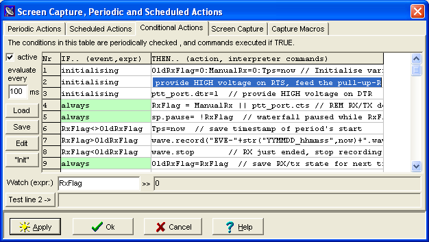
To see or modify the "conditional actions" which perform the tasks mentioned
above, select "File".."Conditional Actions" in SpecLab's main menu. You will
see a table like this (most likely, already changed a bit, because this was
the author's very first attempt) :
-
Note:
-
You will find the "sourcecode" of these event-definitions in the
"conditional_actions" folder, saved as
EVE-RxTxControl.txt. You
don't have to load them manually, because they are are also part of the SL
configuration for the EVE experiment, at least in the file EVE-SDR-IQ-5kHz.USR
. A general description of the conditional actions is
here (in the SL manual) .
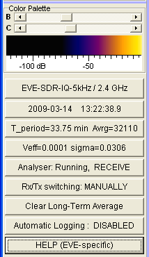
The proper function and the "progress" of the experiment can be checked on
the programmable buttons on the left side of the main window. It shows (from
top to bottom) the current date (YYYY-MM-DD), the current time (hh:mm:ss),
the current time within a 5-minute RX or TX cycle ("Tp=2 min" means the current
cycle is running for 2 minutes now; values above 5 minutes indicate a problem..).
Next, there is a programmable readout for the "effective voltage" within
a certain frequency range (right-click on the button to edit it), and an
indicator for the current RX / TX - state:
-
"Running, Auto" means the analyser is running, audio data are captured in
a wave file, and the system runs "automatic" (no manual RX/TX switching
required);
-
"Paused, Auto" means the analyser is paused (because the transmitter is active,
and the receiver is passive); no audio data capturing, and the system runs
"automatic";
-
"Running, Manual" means the analyser is running, audio data are captured;
but the system has been started MANUALLY (by clicking on this button) - most
likely, because the human operator noticed that "something went wrong" (someone
ripped the cable off, the serial port doesn't work as it should, etc etc).
NOTE: After manually starting the analyser, you must also stop it manually
- it won't stop automatically in this mode !
Note: If the analysis PC (laptop ? AMSAT PC ?) doesn't have a serial port,
bring a suitable USB / RS-232 adapter along for the experiment ! Otherwise,
RX/TX switching must be performed "manually" as explained above. During the
last 10 GHz test, automatic switching was used.
The programmable buttons can be modified by clicking on them with the RIGHT
mouse button. The LEFT mouse button invokes the programmed function (where
applicable; some buttons are used for "display" only).
-
The first button shows the local date and time by default. Like all buttons,
it can easily be reprogrammed if required (right-click on it to open the
macro-button editor).
-
The second button shows the time elapsed in the current receive or transmit
period ("T_period"), and the number of Averages ("Avrg") since the experiment
started. For safety, this button doesn't do anything when clicked - it is
only used as a custom display area.
Note: You can clear the long-term average before starting with the "Clear
Long-Term Average" button mentioned further below.
-
The button "Veff=0.0xx sigma=0.xxx" shows the effective voltage
(veff function) in the last FFT, and
the standard deviation (sigma function)
within the frequency bins in the long-term average spectrum. This is an important
indicator to check if everything works as it should
(*).
-
The button "Analyser: Running, RECEIVE" / "Paused, Transmit" shows the current
state of analyser as explained in the previous chapter.
Clicking this button will stop the automatic receive/transmit cycle (ignoring
the state of the digital control line), and enter manual Rx/Tx mode.
In manual mode, clicking this button toggles between receive (i.e. analyser
active) and transmit (i.e. analyser paused).
To resume "automatic" mode, use the next button.
-
"Rx/Tx switching: MANUALLY" .. / "Rx/Tx switching: Automatic" shows if the
receive / transmit cycle is currently controlled trough the serial port,
or manually. To switch from manual to automatic operation, click on
this button.
To switch from transmit to receive, or from transmit to receive, click on
the button showing RECEIVE or TRANSMIT.
Note: With MANUAL receice/transmit control, the receive cycle doesn't stop
automatically after 5 minutes ! Only if the RX/TX hardware switch doesn't
work, or there is no serial port interface available, use manual control.
-
The button "Clear Long-Term Average" clears the Long-Term Average Spectrum,
details about that function are
here.
Use it ONCE to reset the old average, not during the experiment.
-
The button "Automatic Logging: DISABLED" / .."Enabled" shows the current
state of automatic wave file logging.
"DISABLED" : The 5-minute receive periods are NOT saved as a wave file.
"Enabled" : When next switching from "transmit" to "receive", a 5-minute
recording (as a wave file) will be started.
-
"Help": Should open a web browser to load this document, and jump to this
chapter (works with Firefox, but not with IE 7).
(*) To check if everything works "as it
should", keep an eye on the "Veff"- and the "sigma" indicator during the
RX-periods. Veff should remain constant (within a few percents of the initial
value). If not, check if the AGC in the VHF receiver is turned off, and look
outside .. there may be rain scatter on 10 GHz.
The "sigma" value (standard deviation) should drop permanently, as more FFTs
are added in the long-term average.
The 'sigma'-value should drop during the experiment as explained
here .
(The following only applies to the 10 GHz experiment. It's unlikely to be
a problem on 2.4 GHz).
If you observe rain scatter (or, something else causes the effective voltage
to rises for a few minutes), write down the current time of day. The increase
in broadband noise will most likely not be caused by Venus ! Later, when
analysing all recorded 5-minute-chunks, you can skip that part of the recording.
When analysing files, the files can be selected "individually" by holding
the CONTROL key pressed in the windows file selector box. If you know the
time of the rain-scatter event, you know the filename of the "unwanted
recording", because the name of the wave file contains of the START-date
and -time in the ISO8601 format. For example, EVE-070812_1700.wav is a file
recorded in August 12th, 2007, on 17:00 "PC"-time.
In contrast of rain scatter (where an "unusually strong signal" would add
unwanted energy into the average spectrum), an "overhead" could pass without
scattered 10-GHz signals won't cause much harm, because the energy in the
momentary FFTs would be weaker than stronger.
--... ...-- .... ..