This document describes an experimental "chirp filter", implemented in each of Spectrum Lab's DSP Blackboxes.
Contents
The chirp filter actually compresses a chirped pulse back into a "short, sharp pulse" by means of correlation with a known reference.
There are at least two sample configurations for the chirp filter, contained in the installation archive:
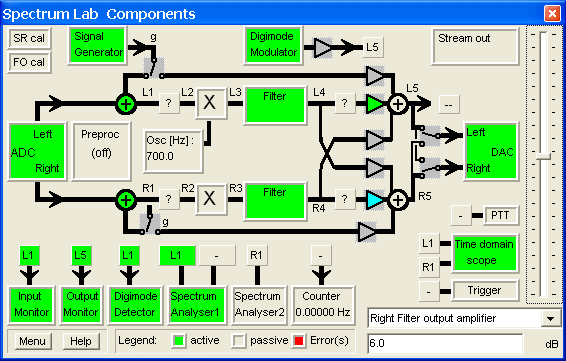
To configure any of the four chirp filters available in Spectrum Lab, open the circuit window, and click on one of the DSP blackboxes (the small squares in the signal paths, usually labelled with a '?') :
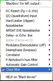
Clicking on a blackbox in this diagram opens a popup menu, in which the blackbox (which includes the chirp filter) can be parametrized:
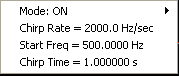
The following parameters can be individually configured for each chirp filter.
Note: Don't make the chirp time longer than necessary, because this may cause a large computational load. Consider this:
To correlate a 1-second reference signal at 48 kSamples/second, the length of the reference signal is 48000 samples. For reasons explained below, the correlator will need calculate a lot of 131072-point-FFTs every 1.73 seconds, which causes a decent CPU load (works ok with a 1.7 GHz CPU, though). It also causes an unavoidable delay of a few seconds between the filter's input and output, dictated by the principle (not by the CPU speed).
To correlate the short 'known reference' with an endless, continuous signal uses a technique known as 'overlap-save' or 'overlap-scrap', which is frequently used to implement very long FIR filters (using the forward and inverse FFT). The principle is as follows:
Sounds like overkill ? Consider this: If we were to correlate a one-second reference signal at 48000 samples/second directly (entirely in the time domain), 48000 points would have to be correlated for each input sample. Because the chirp reference signal is complex, this requires 2*48000 floating point multiplications per input sample(!), or 2*48000*48000 = 4608 million multiplications per second ! The FFT-based correlation is much more effective for 'long' reference signals, but it still has its limiations. On the author's 1.7 GHz Centrino Duo (notebook), a 1-second chirp at 96 kHz sample rate was impossible to process (continuously, in real time).
This configuration was added 2010-02 for experiments with a bistatic(*), chirped, backscatter radar for amateur radio use on HF or VHF. It is based on ideas presented by Andrew Martin (VK3OE) on the VK Logger forum .
To use this configuration, select Quick Settings .. Other Amateur Radio Modes .. Chirp Radar Receiver from Spectrum Lab's main menu. If you have a software defined radio like SDR-IQ or Perseus, select that device for input (instead of the soundcard) after loading. The time domain scope was used as a 'graphic frontend' for the radar receiver.
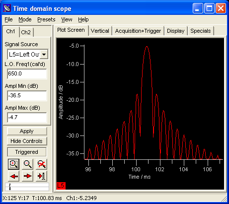
The chirp is 1 second long, endlessly repeated, and sweeps from 500 Hz (audio) to 2500 Hz. At the receiver site, it is de-chirped with one of the chirp filters (part of SL's DSP blackboxes). The curve above shows the chirp filter's output in the time domain (on the time domain scope). The chirp was compressed into a pulse which is less than a millisecond wide. More 'compression', resulting in a better spatial resolution could be achieved at higher sampling rates, and larger frequency sweep ranges (which is impossible with a normal "SSB" transceiver with 3 kHz bandwidth). The periodic chirp can be generated by a dedicated, or with SL's test signal generator. To turn the 'Transmitter' (chirp generator) on or off, click on the programmable button labelled 'Radar: Receiving' / 'Radar: Transmitting'. It toggles between receive and transmit. The TX-signal will be fed to the soundcard's output. You can use this for off-air-tests with the PC's speaker and microphone (acoustic radar).
As long as we don't know the precise timing of the transmitted pulses, the time domain scope's display buffer must be made large enough to capture one second of data (which is the chirp radar's repetition interval). Initially, after starting the chirp 'receiver', zoom out to see the entire 1-second interval on the scope's screen.
Hopefully you will find the 'direct' pulse (which took the shortest path from transmitter to receiver, usually the line-of-sight). Depending on the location and conditions, this pulse will be the strongest of all, and also be the most narrow pulse (least dispersion). If you cannot spot the 'direct' signal, make a guess, or wait until a more sophisticated way to synchronize the transmitter and receiver has been developed ... something like GPS locking or similar.
After identifiying the pulse with the direct signal, zoom into the important range. To do this, drag a marker frame with the mouse around the 'interesting' area, with the leading pulse on the left edge of the marker.
When releasing the mouse button (after dragging the red marker frame), a popup menu opens in the scope's graphic window. Select the item 'Zoom in (into selection)'. The time domain graph will be redrawn, zooming in on the marked area. You can also fine-tune the horizontal and/or vertical scroll position as explained here .
If the soundcard's sampling rate has been properly calibrated, the position of the display should not 'wander around' while the receiver keeps running. If it does, try to calibrate the soundcard's sampling rate as explained here.
By default, the 'Chirp Radar' configuration uses a logarithmic dB scale, with 0 dB = "full scale". You can modify this (for example, use a linear scale) in the time domain scope settings. The chirp filter itself always produces a linear output (proportional to the input).
<ToDo: Complete this....>
See also: Spectrum Lab's main index , time domain scope , programmable frequency markers , spectrum displays , main frequency scale .