 |
|
|
|
Introduction
The introductory paragraphs in the ealier article gave an explanation of why there is a need to check the balance of currents in the transmission line. The explanation is repeated in the appendix at the end of this article.
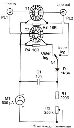
The original circuit of the balance meter (and also the new circuit) consists of a current transformer in each leg of the line. In the original circuit the two line leg currents were simply compared. There has been some criticism concerning whether the simple comparison was adequate to assess the degree of balance (or unbalance) on the line. The arrangement in the new circuit is a different measurement in terms of comparing the relativity of the longitudinal current component with that of the differential current component.
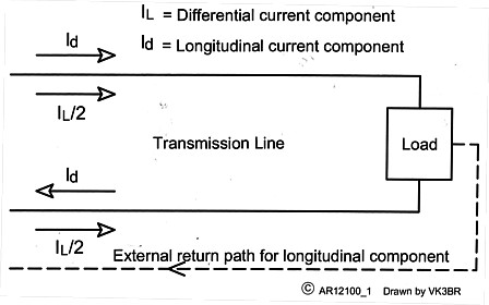
The differential current is the normal current component which flows in a balanced circuit or line. Current flows in one leg of the line and returns in the other leg, the same amplitude as the first leg but in opposite phase. (Shown in the diagram Figure 1)
The longitudinal or common mode current component can be considered to flow equally in both line legs and in phase. In real terms it may be more complex than this, but for the purposes of the readings from this instrument, that is how the currents are analysed. The generation of a longitudinal component generally results from a return path to the source outside of the two line legs. (Also shown in the diagram Figure 1)
The presence of both longitudinal and differental components normally results in an unbalance of the currents in the two legs of the line. Measurement of these two currents was the method of unbalance detection used in the original circuit.
|
Basis of the new Circuit To explain how the circuit works, we turn to a few mathematical expressions: Referring to the original circuit (figure 2), the two line leg currents can be expressed as follows: Let Id = differential current in the line at a reference phase of 0 degrees in one line leg, |
|
The longitudinal or common mode component IL can be expected to be at a random phase relative to that of the differential current component. So we express that in complex form and we let IL = (Ica + jIcb).
(Its amplitude and phase relative to Id is dependent on the line location that the measurement is made).
The longitudinal current component is shared between the two legs and the current in each leg is equal to (Ica + jIcb)/2.
The current flowing in one leg of the line (as measured by the meter) is the result of: [(Ica + jIcb)/2 + Id].
And the current in the other leg (as measured by the meter) is the result of: [(Ica + jIcb)/2 - Id] (Note that the differential component Id in one leg is reversed in phase to the other leg).
Voltages are developed across the two 18 ohm resistors R3 and R4 equal to the currents in the two legs multiplied by a constant C.
If the two voltages are added by direct mathematical addition, we get [(Ica + jIcb) x C] and the differential component Id is cancelled out.
If one of the voltages is phase reversed and the two voltages added, the longitudinal component (Ica + jIcb) is cancelled out and the result is (2Id x C).
The modified Circuit
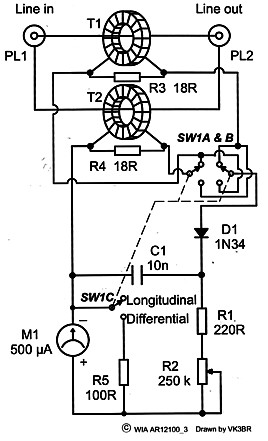
So all we need to do to compare the longitudinal and differential current components is to connect the two voltage outputs across the two 18 ohm resistors in series and provide a switch (SW1AB) to select phase reversal of one of the two voltage outputs. One position of the switch selects a meter reading which is a function of the differential current multiplied by 2. The other selects a meter reading representative of longitudinal current relative to the differential current. To correct for the multiplication by two of the differential current, a third section of the switch (SW1C) connects in a shunt resistor to halve the meter reading for the differential position.
Figure 3 shows the circuit modified for reading relativity of Longitudinal to Differential currents. All that is required is the replacement of the SPDT switch with a 3PDT switch and some re-arrangement of the wiring.
|
|
Meter Readings
|
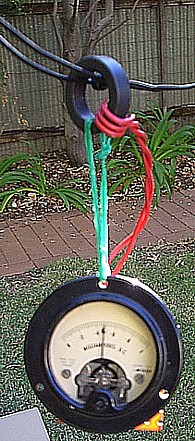
Standing Waves on the Longitudinal Current component over the length of Line It is almost certain that if the line length is considerable compared to a wavelength, standing waves will be set up in the longitudinal current component and nodes and anti-nodes of current will be formed. So the actual longitudinal current will depend on just where it is monitored as well as the degree of unbalance in the transmission line circuit. Probably the easiest place to take the measurement is at the transmitter source connection to the line. However there is the possibility that this place also could be a node in the developed longitudinal current. In this case, the metered longitudinal current could read low and one could be misled into thinking that the line circuit was well balanced. If this is suspected, a toroidal current transformer coupled to a detector (as shown in figure 4) could be run down the whole line pair (or coax) for about 1\8 to 1\4 of a wavelength to detect where the nodes and anti-nodes might have occurred. If a node is located at the test point, it might be suitable to shift the location of this node by the temporary addition of a length cable in series with the line. Alternatively, one might just add about 1\8 wavelength of cable anyway and compare the metered result with and without, the added cable. Of course, because of the variation of current along the line, these tests will simply give an indication of whether the longitudinal current component is considerable compared to the differential current component, or whether it is small enough to be ignored. If a more specific record is desired, I suggest an anti-node or point of maximum longitudinal current be located and record the relativity of the longitudinal to differential currents for that point. |
|
Measurement to assess of balance at the output of a Source
Whilst the test unit was made to examine the relativity of the longitudinal current component to the differential current component on transmission lines, it can also be used in the same way to assess the degree of balance in the output of an RF source (such as the balanced output of a radio transmitter or an antenna tuner).
To set this up, feed the balanced source into the input of the test unit and terminate the output of the test unit in two series load resistors each equal to half the nominal load resistance of the balanced source output. Connect the centered junction of the two load resistors to the ground reference of the source. Power in the region of at least 10 watts of power is required to operate the test unit and the load resistors need to be rated for that power.
The test unit is built nominally for the HF bands and it is assumed that the length of leads between the source and the load would be a mere fraction of a wavelength. As such there should be no problem with standing waves and current nodes as discussed in the previous paragraph.
The balance of the source can be assessed in terms of the ratio longitudinal to differential currents as measured.
Conclusion
Modifications to the original Transmission Line Balance meter (AR Aug/Sept 2009) which simply compared the two line leg currents, have produced a new meter which compares the longitudinal (common mode) current component on the line with the differential current component.
In assessing measurements, either with the original balance meter, or with the new circuit arrangement, one should not overlook the effects of the standing wave which may well occur in the longitudinal current component over the length of the line.
The test meter might also be put to use to assess the balance performance of the balanced output of a transmitter or antenna tuner.
Reference
"A Transmission Line Balance Meter" by Lloyd Butler VK5BR, Amateur Radio, August/September 2009. -
also http://users.tpg.com.au/ldbutler/Line_Bal_Test_Meter.htm.
Appendix
Introduction in the Original Article on the Line Balance Meter
A typical amateur radio antenna installation makes use of a simple dipole or other balanced form of antenna fed via a coaxial transmission line. Because the line is unbalanced, some form of unbalanced to balanced coupling is normally necessary between the coaxial line and the antenna. Without this coupling, a condition is set up where currents running in the inner and outer legs of the coax line are unbalanced and a common mode or longitudinal current component is developed along the length of the line, causing radiation from the line. Apart from distorting the radiation pattern inherent to the antenna proper, it encourages annoying induction into equipment and wiring within the radio shack, as well as on receiving, encouraging induction of vertically polarised near field noise.
A typical balancing interface is the choke balun which must have sufficient common mode rejection impedance to minimise the longitudinal current component. Whilst most radio amateurs possess an SWR meter which can be used in series with the coax line to check how well the antenna is matched to the 50 ohm line, it gives no indication that the currents running in the two legs of the line might be unbalanced. The SWR meter can show a perfect 1:1 SWR indicating that the antenna is loading the line with a resistance of 50 ohms. However with such a condition indicated there can still be a high longitudinal component flowing and radiation from the line.
Whether there is a serious unbalance of currents in the line legs can easily be checked by measuring the two currents. However it doesn't seem to be something which is routinely done in checking out the antenna system and verifying whether the coupling interface (such as the choke balun ) is adequate for the job.