 |
|
|
|
|
Introduction
The article discusses the theory of loop aerials for receiving and how they reduce the level of local noise. A Loop Aerial is described suitable for use on the LF and VLF bands together with a circuit of an interface loop tuner and preamplifier. The discussion extends to the problems of amplifier noise and the advantages of tuning the loop.
Loop Aerial Theory
A major problem in receiving VLF and LF signals is the high level of local noise generated from noisy power lines and consumer electrical equipment. In the presence of this type of noise, the received signal-to-noise ratio can be improved with the use of a loop aerial.
To explain this, it is necessary to briefly discuss the fields around a radiating element. At distances up to around half a wavelength, the induction or near field is prominent but it falls away at a greater rate with distance than the radiation field. At distances greater than one half wavelength, the radiation field is prominent. The relationship between field strength and distance is as follows:
1. The electric component of the induction field decreases with the cube of the distance and dB = 601og (d2/d1) where d2 and d1 are the relative distances.
2. The magnetic component of the induction field decreases with the square of the distance and dB = 40log (d2/d1)
3. Both the electric and magnetic components of the radiation field decrease directly with distance and dB = 20log (d2/d1)
The effect of all this is that, in the near field, the electric
component is much stronger than the magnetic component. This is
illustrated graphically in Figure 1.
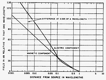
At VLF and LF (10 to 300 kHz) we are concerned with half wavelengths between 500 and 15,000 meters, and reception of localised noise is clearly in the induction or near field region. The loop aerial is essentially sensitive only to the magnetic component, and because this is lower in level than the electric component in the near field, the level of noise interference is reduced. Furthermore, if the source of interference is from a different direction than that of the signal to be received, the noise is further reduced by the directional properties of the loop. The loop has a very sharp null at right angles to the plane of the loop and can be rotated to position the noise source at the null.
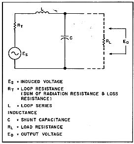
The equivalent circuit of the loop aerial coupled to a load
resistance (RL) is shown in Figure 2. Es is the voltage induced
into the loop, RT is the resistance of the circuit (the sum of
radiation resistance and loss resistance), L is the inductance of
the loop, C is the shunt capacitance of the loop with its cable
coupled to the load and Eo is the output voltage across the
load.
When the loop plane is in line with the direction of the signal
for maximum signal level, induced voltage Es is given by the
following formula (valid providing the loop dimensions are small
compared to a wavelength):
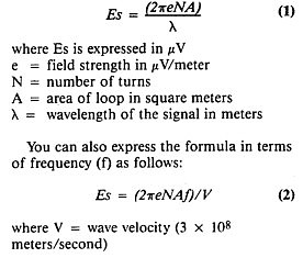
From the formula, it is clear that the induced voltage is directly proportional to both the loop area and the number of turns. The larger you make either of these, the higher the induced voltage. However, increasing these also increases the series inductance and shunt capacitance and, depending on frequency, their reactances have a profound effect on the actual voltage Eo delivered to the load. Resistance RT is also in series with the load, but its value is normally low enough to make little difference to the voltage delivered to the load.
Resonance
The loop aerial has a natural resonant frequency at which the reactance of L equals the reactance of C and at which the response peaks such that the output voltage, Eo, equals the induced voltage, Es, multiplied by the Q factor of the circuit. Clearly, there is much to gain by operating the loop in a parallel-tuned mode. This can be achieved at any frequency lower than the natural resonant frequency by simply adding shunt capacitance across C. At frequencies above the natural resonant frequency, resonance is not possible. Good performance is then better achieved the by decreasing the number of turns on the loop to make natural resonance equal to or above that of the frequency used.
To obtain good performance in a resonance mode at a wide range of frequencies, a number of loop aerials with different numbers of turns, or one with a selected number of turns, is needed. At low frequencies, a large number of turns is desirable to achieve good signal sensitivity. At higher frequencies a lesser number of turns might have to be used to raise the natural resonant frequency. Referring back to Formula 2, you will see that induced voltage Es is proportional to both the frequency and number of turns, so while you lose signal level with less turns, this tends to be compensated for by the increase in frequency.
As output voltage,Eo is proportional to the Q factor at resonance, it is important to make load resistance RL a high value to prevent the lowering of Q. This calls for coupling directly into an amplifier with a high impedance input.
Shielded loop
Whilst the loop aerial essentially operates on the magnetic component, there can be a residual pick up of electric component. For Direction Finding use, it is important to electrically shield the loop to minimise the electric field induction. In practical use for just receiving at LF-VLF, there seems to be little to gain by the small reduction in electric pick-up. In fact shielding increases the residual capacitance of the loop and reduces the maximum tuning frequency for a given number of turns.
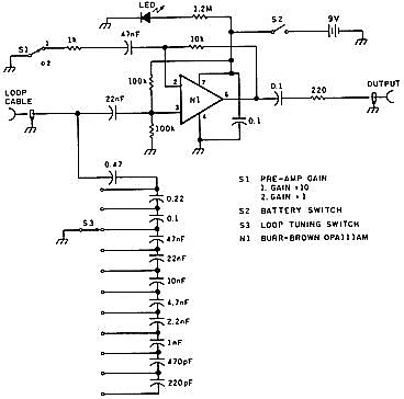
Loop Interface
The dynamic impedance of the tuned loop can be very high, hence
the circuit must be interfaced with the high impedance input of an
operational amplifier or a FET stage. Figure 3 is the circuit of an
amplifier that has been used by the writer. The amplifier is set
for a maximum gain of 10 to increase further the signal level from
the loop which, even with tuning, produces a much lower signal than
that received from a random wire of reasonable length. The
amplifier is provided with a switch to reduce its gain to unity in
the event of very high signal levels causing cross modulation.
Sometimes there is an advantage in balancing out any residual vertical pick-up using a balanced amplifier input. For another circuit using a balanced input, CLICK HERE. This is desrcibed in another article on 1.8 MHz receiving Loops.
Amplifier noise
When operating VLF-LF using a wire aerial, the atmospheric noise level received is normally well above the noise floor of the first amplifier, and amplifier noise is insignificant. With the loop aerial, the signal pickup is much lower, and when the atmospheric noise level is low, the minimum discernible signal level can be set by the amplifier noise floor rather than the atmospheric noise level. It is therefore important to select a preamplifier with a low inherent noise, much as one would do for a VHF or UHF front end.
For the amplifier used in the circuit of Figure 3, a Burr-Brown low-noise FET operational amplifier type OPA111AM was selected. This is specified as having the low voltage noise figure of 6 nV per root hertz of band width, with the negligible current noise characteristic of the FET input circuit. It has a gain-band width product of 2 MHz and hence it can maintain the gain of 10 up to a frequency of 200 kHz with a falling response at higher frequencies down to a gain of 4 at 500 kHz.
Another choice for a low-noise amplifier could have been the bipolar input Precision Monolithics type OP27 amplifier. This has a voltage noise of only 3 nV per root hertz of band width but, having a bipolar input, there is a current noise component which would add noise when connected across the high impedance tuned loop circuit (ref 2). The amplifier has a gainband width product of 8 MHz and hence could maintain the gain of 10 well up to 800 kHz. A further approach might have been to use one of the low-noise MOSFET VHF transistors such as the BF981.
Of course, good signal-to-noise ratio also gets back to the design of the loop for highest possible signal voltage. Recapitulating previous parts of this discussion, signal voltage is increased with more turns or larger area (consistent with natural resonance being not less than the operating frequency), or by designing the form of the loop for the highest possible Q factor.
Loop aerial circuits are frequently published with an amplified signal fed back to the loop to form what is called a Q multiplier. This, of course, is a different name for what has been known as regeneration or reaction. Feedback in phase with the input signal raises the effective Q of the circuit to increase its gain and reduce its band width.
There is also a disadvantage with using regeneration in that the noise generated by the amplifier is also fed back to be re-amplified. While the regeneration narrows the loop band width and reduces the band width of the incoming noise, it actually increases the level of the amplifier noise within the band. However the writer has found that regeneration is quite useful at LF frequencies to restrict the front end bandwidth and increase sensitivity. (Refer to Active Loop article).
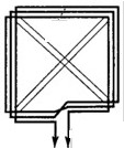
A Typical Loop Aerial
The natural resonant frequency of the loop and hence its upper frequency limit for a given number of turns, can be increased by spacing the wires and spacing the shield from the wires so that residual capacitance is reduced. With this arrangement, the residual capacitance can be reduced to provide a considerable increase in the upper frequency of the loop.
Good results have been achieved by a loop assembled by the
writer (refer figure 4). This consisted of 20 turns of 1 square mm
hook-up wire spaced laterally 10mm apart on a wood frame 0.8meter
square. To achieve the spacing, the wire was wound around four
pieces of doweling fitted through two wood cross pieces. This
aerial measured an inductance of about 500 uH and had a natural
resonant frequency close to 500kHz. This sets the highest tuneable
frequency which allows tuning of Aeronautical Non Direction Beacons
which are on frequencies of 200kHz upwards.
Amateur bands have been allocated in some countries (such as New Zealand) in the region of 160 to 190 kHz. If operation is confined to no greater than these frequencies, a lower natural resonant frequency can be tolerated and the loop dimensions increased. A suggested loop of similar construction is 28 spaced turns on a 1 metre square frame. Maximum tuneable frequency for this one is around 200 kHz.
The higher one can make the loop Q, the greater its signal sensitivity and its ability to present a signal level which can override the interface amplifier noise. Q can be improved by using as heavy a gauge wire as can be obtained. Signal level is also increased by increasing the number of turns or the area of the loop but increasing either is limited to the point where natural resonance is just above the operating frequency.
Concerning the choice of increasing turns or increasing area, an article from Break-In, July 1997 (ref 4). discussed this issue relative to the loop noise generated by its own loss resistance. The writers point out that the ratio of signal level to noise generated by the loop is improved by increasing area but increasing turns makes no difference to this ratio. Concerning the New Zealand LF band, the writers also say that to ensure that the noise floor is set by atmospheric level and not the loop itself, the diameter of a circular loop should not be less than 1 meter.
Measurement of loop constants
At this point, it might be useful to explain how the loop constants were measured. Having constructed a loop aerial, you need to know its natural resonant frequency and its self inductance so the maximum tuneable frequency can be determined and the capacitance values worked out for the tuning range required. These factors can be measured using a signal generator fed via a fairly high resistance (say 10 k) to the loop as shown in Figure 5. More than one signal generator might be needed to tune from VLF to ME The voltage across the loop is monitored on a CRO (or perhaps a VTVM) via a high impedance probe. The signal generator frequency is adjusted for a peak in voltage at which the natural frequency is indicated. You now add a large capacitance (at least 20 nF) sufficient to make the loop capacitance insignificant by comparison, and retune for a peak at the new lower frequency. Inductance is then calculated from the normal resonance formula (or a resonance chart), using the parallel capacitance as the value of C and ignoring the self-capacitance of the loop as this makes little difference to the accuracy of calculation.
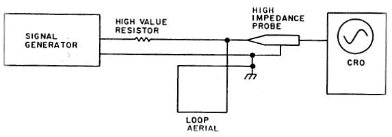
Having measured the self-resonant frequency and calculated the inductance, the loop self-capacitance can also then be derived from the resonance formula.
As a further operation, Q factor can be measured using the same equipment, except that the resistance in series with the signal generator must be increased to around 500 kohm to prevent the Q being lowered by the signal source. With extra signal loss across the resistor, a high signal level and a sensitive CRO are needed. The procedure is simply to measure the frequencies either side of resonance which give 0.707 of the voltage at resonance. The Q factor is equal to the resonant frequency, divided by the difference between the two frequencies recorded. The Q factor at a range of frequencies can be carried out by varying the value of the shunt capacitor to obtain resonance at each of the frequencies.
To go one step further, you can now calculate the AC resistance of the loop (Rt) at any frequency for which you have derived Q. The inductive reactance at that frequency is calculated from 2PifL and the reactance is then divided by Q to obtain Rt. You now know all the constants Rt, L, and C, as shown in Figure 2.
Performance
Whilst the level of its signal pickup is low compared to the long wire aerial, the loop aerial can separate out signals in the presence of localised noise which overrides the signal on the long wire. As with any directional aerial, it also improves the signal-to-noise ratio for atmospheric noise by restricting noise received -in particular from a direction at right angles to its plane.
With a suitably designed loop aerial and highly selective front-end tuning system, good signals at VLF and LF can be received even indoors-right down to 10 kHz. This is gratifying if one does not have room for an outdoor aerial. Of course, there are the odd traps. It is very easy to miss a signal if it happens to arrive from a direction close to the null of the loop. It is also very easy to home in on some inside-based signal source such as a frequency counter.
Untuned loop
Discussion has been centred around loop aerials tuned to resonance and giving output voltage as in Formula 1 or 2 multiplied by Q. However, loop aerials can also be operated in a broadband mode and a design procedure for doing this over a range of frequencies is described in the April 1989 issue of Lowdown (ref 3). The procedure is to load the loop aerial into a fairly low resistance at the preamplifier input, equal in value to the loop inductive reactance at the lowest frequency of the frequency band required. Parallel resonance is set to a frequency calculated from the geometric mean of the lowest and highest frequency required. According to the article, the design produces a loop response which is flat with frequency.
Whilst the broadband loop eliminates the complication of loop tuning when changing frequency, the loss of Q multiplication can drop atmospheric noise below the noise floor of the amplifier, thus limiting the sensitivity to weak signals. As an example, if we apply Formula 2 to the 12-turn 0.8meter square loop described, and use a typical atmospheric noise for 100 kHz, which can be around 0.2 uV per meter per root hertz, we get a loop output voltage of 3.2 nV per root hertz. This output level is barely comparable with equivalent input noise voltages at low impedance of the best of amplifiers.
Conclusions
A properly designed loop aerial system, with a low-noise preamplifier, is a useful part of the VLF-LF receiving equipment and can enable signals to be picked out from noise which otherwise overrides the signal from the wire aerial. It also provides a means to obtain good signal reception at VLF-LF without the use of a large aerial installation usually considered necessary for low frequency reception.
The signal level received from the loop aerial is low compared to the wire aerial and the signal-to-noise ratio can be limited by the noise generated in the first amplifier. To minimize this problem, a low-noise preamplifier is used, and the loop circuit is tuned so that the signal level into the amplifier is multiplied by the Q factor of the loop circuit.
Some experimental loop aerials and a loop tuning and interface circuit have been described.
Following articles (Just Click)
Additions to Active Loop Converter for VLF
REFERENCES
1. Lloyd Butler, VK5BR, "A VLF-LF Receiver," Communications Quarterlv, Winter 1991
2. Lloyd Butler, VK5BR, "Amplifier Noise," Amateur Radio, November 1982.
3."Analysis & Design of Broadband Low Frequency Loops," Lowdown, April and May 1985.
4. LF Scene - Andrew Corney ZL2BBJ and Bob Vernall ZL2CA, Break-In, July 1997.
BIBLIOGRAPHY
1. Direction Finding - Handbook of Wireless Telegraphy Section 7.