 |
 |
After constructing my Elecraft K2/100 transceiver in May 2003, I found myself in need of an accurate frequency reference to calibrate my transceiver's 4 MHz reference oscillator. I expected to be able to reference the 5th harmonic of the oscillator to that of WWV's 20 MHz transmitter, but reception of WWV was non-existent at the time due to low sunspot numbers and generally poor summertime HF propagation conditions. As a result, I began thinking about designing a reliable, high quality frequency standard for calibrating my K2 and for other projects that would function independently of sunspots, time of day, seasons, or critical propagation conditions.
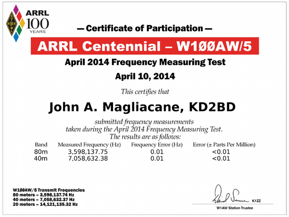
Later that year, the American Radio Relay League announced plans to conduct a Frequency Measurement Test, where participants would be ranked in terms of how accurately they could measure W1AW's operating frequency. The prospect of participating in the 2003 FMT provided yet another incentive for developing a highly accurate frequency standard.
|
|
I was successful in developing a simple WWVB-disciplined frequency standard and using it in concert with my K2/100 transceiver and Heathkit frequency counter to participate in the 2003 ARRL Frequency Measuring Test and yield respectable results.
However, an engineer's work is never done. No matter how swift or clever an engineer's design, it can always be improved.
As such, my FMT methodology has evolved significantly since my original involvement in 2003, and currently employs electronics that is completely self-engineered. The results I obtain using this "homebrew" approach are often superior to those of many well-experienced FMT participants who employ commercially manufactured laboratory-grade instrumentation costing many thousands of dollars.
In between FMTs, my frequency measurement hardware is often used to study the behavior of the Earth's Ionosphere. This is done by measuring the frequency of standard radio broadcasts provided by radio stations CHU and WWV, and measuring the Doppler effects imposed on these signals by the ionosphere. It is my hope that knowledge can be gained through these studies that might lead to even higher accuracy frequency measurements in the future, or perhaps a sobering realization that we can do no better.
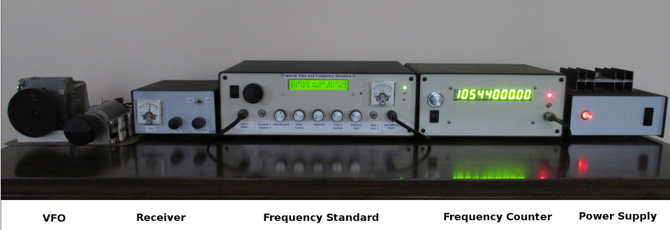
What follows is a brief history and description of the FMT hardware I have developed and employed over the past decade, along with the results of ionospheric studies that illustrate some of the perturbations that make accurate, long-distance frequency measurements somewhat challenging, to say the least.
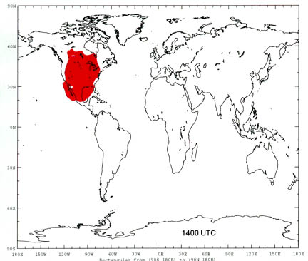
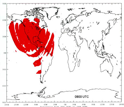
Frequency measurements, calibration procedures, and even the proper tuning of musical instruments are made with reference to known and trusted frequency standards. In the United States, the National Institute of Standards and Technology (NIST) provides wireless broadcast distribution of standard audio and radio frequencies through radio stations WWV, WWVB, and WWVH. While WWV (Colorado) and WWVH (Hawaii) operate on shortwave frequencies whose reception is greatly influenced by the Earth's Ionosphere, WWVB (co-located with WWV) operates on a much lower frequency of 60 kHz, whose propagation is influenced by ionospheric instability to a significantly smaller degree. In fact, so accurate and reliable are the reception of WWVB's broadcasts, that they have been widely used as a frequency reference in the scientific and engineering communities for many decades.
Contours provided by NIST illustrate that WWVB broadcast coverage is far more reliable than that possible on short-wave frequencies:
 |
 |
Attempts made to receive WWVB using a multi-turn resonant loop antenna, 40 dB gain preamplifier, and oscilloscope confirmed that reliable reception was indeed possible in New Jersey, 24 hours a day, and as such might serve well as a frequency reference:
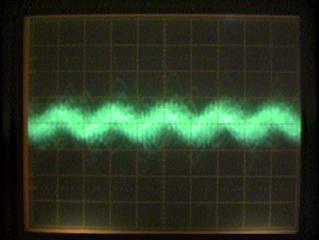
My successful reception of WWVB using this simple hardware was officially confirmed by the National Institute of Standards and Technology (NIST), adding further encouragement for the subsequent development of a WWVB-disciplined frequency standard:
 |
 |
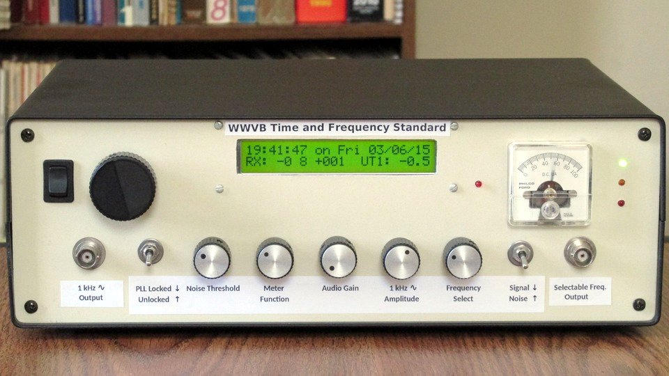
My frequency standard would eventually take the form of a carrier phase tracking receiver that would discipline a 10 MHz voltage-controlled temperature compensated crystal oscillator (VCTCXO) with reference to WWVB's 60 kHz atomically controlled carrier. Synchronous demodulation and correlation decoding techniques employed previously in my KD2BD Pacsat Modem (published in August 1994 QEX), were used to good advantage in this application to reliably demodulate WWVB's amplitude shift keying under the influence of noise.
Processing and decoding of WWVB's legacy time code were implemented using a Microchip PIC16F88 microcontroller that (among other things) functions as a real-time UTC clock, controls 60 kHz RF phase shift circuitry that compensates for WWVB's hourly phase signature, provides UTC date, time, UT1 correction, and PLL error voltage information to the user through an LCD display, and sends time and date information in the form of a serial data stream for accurately synchronizing a data logging PC to the current time. Harmonics and sub-multiples of the 10 MHz VCTCXO derived through decade counters provide a wealth of local reference signals for frequency measurement and calibration purposes.
The introduction of BPSK modulation to WWVB's broadcast format in 2012 forced modification of the receiver's basic design from that of a phase-locked loop to one of a Costas Loop.
An audio clip demonstrating the reception quality this receiver delivers 1622 miles east of WWVB can be found here. A technical article describing the design and operation of my frequency standard was published in the November/December 2015 issue of QEX magazine. A PDF version of my article is available here.
Distant radio signals of unknown frequency are received using a quadrature phasing (imaging rejecting) direct conversion receiver of my own design. My receiver employs a pair of doubly balanced mixers driven by the I and Q outputs of a digital phase shift network that is driven by an AD9851-based Direct-Digital Synthesis (DDS) variable frequency oscillator (VFO) operating on a frequency close to four times that of the incoming signal.
My receiver possesses a 50 Hz wide passband that is centered on an audio output frequency of exactly 1000 Hz. This high level of selectivity, and the majority of the receiver's sensitivity, are obtained through active bandpass filters designed around low-noise operational amplifiers.
The front end RF amplifier and VFO circuitry are housed separately from the receiver's enclosure, permitting easy substitution of these systems depending on the specific application of the receiver.
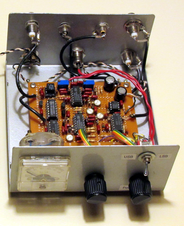
The tuning procedure begins with resonating the antenna and the receiver's front end to the approximate frequency of the signal being measured. The VFO is then carefully tuned until the desired signal is found and demodulated by the receiver as a 1000 Hz audio tone.
Audio from the receiver is mixed along with a 1000 Hz reference tone produced by the frequency standard in a phase comparator. The phase comparator produces an "error voltage" proportional to the phase difference between the two 1000 Hz tones. The error voltage is filtered and applied to a 30 MHz VCXO that serves as the clock for the DDS VFO, thereby electronically steering the VFO toward a frequency where the distant radio signal is demodulated as an audio tone of exactly 1000 Hz, and holds the VFO locked in phase with reference to the signal to be measured.
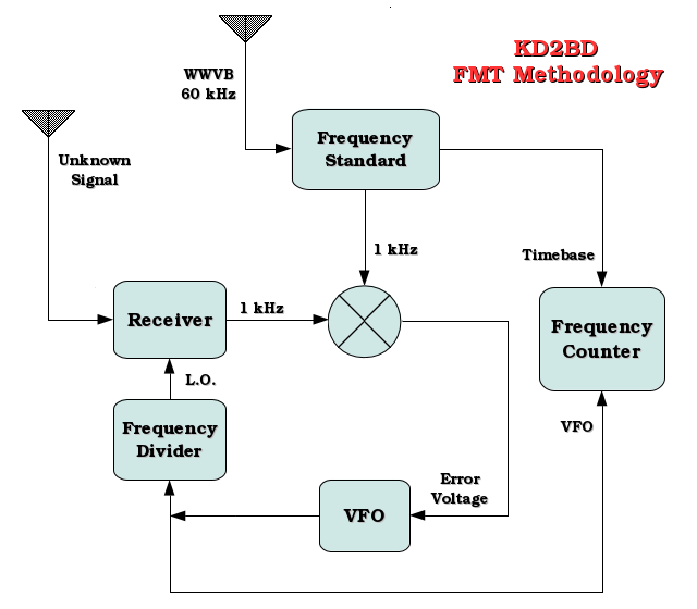
Once this phase locked tuning arrangement has been established, the frequency of the receiver's VFO tracks the frequency of the distant radio signal through a very specific offset. Careful measurement of the VFO's frequency, followed by compensation for the offset, yields the frequency of the distant signal to a very high degree of accuracy.
The frequency of my receiver's VFO is measured using a 10 digit frequency counter of my own design. The frequency counter operates by gating a sample of the VFO into a string of 74HC4040 ripple counters, the first being a member of the Fairchild 74VHC very high speed CMOS family.
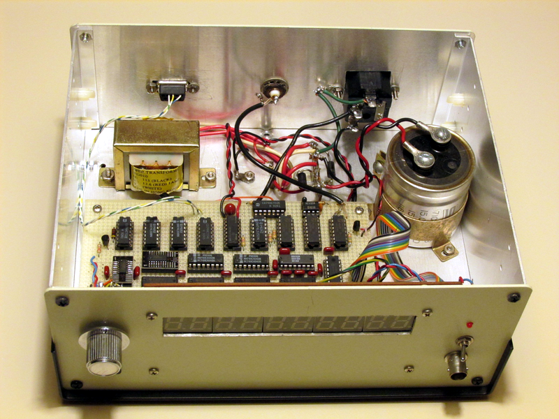
Gating periods of 100 seconds, 10 seconds, 1 second, and 1 millisecond are available, and are under the precise control of the WWVB-disciplined frequency standard. Front panel controls allow the frequency measurement process to be aborted and restarted at any time.
After the gating period has ended, the count accumulated in the ripple counters is latched in a series of parallel-to-serial shift registers and serially transferred to a PIC16F88 microcontroller. The microcontroller assembles the 32-bit serial data stream into four 8-bit words, converts these binary words to BCD, and sends the result to a 10 digit LED display as well as a Linux-based PC through an RS-232 serial data connection.
If the frequency counter is configured for a gate period of 100 seconds, it can resolve a frequency measurement down to the nearest 0.01 Hz (10 milliHertz). However, the resolution of FMT measurements are enhanced beyond that amount by taking readings directly at the VFO prior to the frequency division taking place in the receiver's digital phase shift network. Since the phase shift network divides the VFO frequency by 4, the resolution of the FMT measurement is increased to 0.0025 Hz (2.5 milliHertz).
When measuring low RF frequencies, binary frequency dividers can be inserted between the VFO and the receiver while keeping the frequency counter directly connected to the VFO. With the VFO operating at 14,064,000.00 Hz and the VFO's frequency divided 4 times above and beyond that taking place in the receiver itself, the frequency measurement of the unknown signal becomes 880,000.00000 Hz with a resolution of 0.000625 Hz (625 microHertz).
That's a resolution of less than one part per billion!
Knowing that the receiver's digital phase shift network divides the VFO frequency by four, and that the receiver demodulates the incoming signal as a 1000 Hz tone, if upper sideband (USB) phasing is employed, the local oscillator injection to the receiver's product detector will be exactly 1000 Hz below that of the incoming signal. Therefore:
Frequency of on-air signal = (VFO Frequency / 4) + 1000 Hz
If lower sideband (LSB) phasing is selected:
Frequency of on-air signal = (VFO Frequency / 4) - 1000 Hz
Example: Suppose the receiver is configured for USB phasing, and the frequency counter reads 13,316,000.00 Hz when the VFO is phase locked to the incoming carrier. What is the frequency of the unknown signal? Answer: 3,330,000.00 Hz.
The carrier of radio station WCBS appears to be referenced to a GPS standard by virtue of the following readings taken within ground wave coverage of the station. Note that these readings were taken throughout WWVB's phase signature period (HH:10:00 to HH:15:00) with no apparent effect on the readings. (That observation speaks very highly of the phase signature compensation circuitry in my frequency standard.)
WCBS - New York, NY - 880 kHz: Sun Jan 06 16:09:37 2008 UTC: 880000.000000 Sun Jan 06 16:11:27 2008 UTC: 880000.000000 Sun Jan 06 16:13:17 2008 UTC: 880000.000625 Sun Jan 06 16:15:07 2008 UTC: 880000.000000 Sun Jan 06 16:16:57 2008 UTC: 880000.000625 Sun Jan 06 16:18:47 2008 UTC: 880000.000000 Sun Jan 06 16:20:37 2008 UTC: 880000.000625 Sun Jan 06 16:22:27 2008 UTC: 880000.000625 |
The slight inconsistency in the readings is due to the +/- 1 LSD error inherent in the digital frequency counting process. This can be reduced through averaging a number or readings over time, the error being reduced by the square root of the reciprocal of the number of periods measured.
WFAN - New York, NY - 660 kHz: Sun Jan 06 17:25:36 2008 UTC: 660000.000000 Sun Jan 06 17:27:26 2008 UTC: 660000.000000 Sun Jan 06 17:29:16 2008 UTC: 660000.000000 Sun Jan 06 17:31:06 2008 UTC: 660000.000000 Sun Jan 06 17:32:56 2008 UTC: 659999.999375 Sun Jan 06 17:34:46 2008 UTC: 660000.000000 Sun Jan 06 17:36:36 2008 UTC: 660000.000000 Sun Jan 06 17:38:26 2008 UTC: 660000.000000 Sun Jan 06 17:40:16 2008 UTC: 660000.000625 |
The second table lists measurements taken of another local GPS-referenced radio station carrier. In this sequence of readings, the LSD count uncertainty quickly averaged out to zero.
Changes in the effective height of the Earth's Ionosphere, variations in layer density, Faraday rotation, and perturbations caused by Traveling Ionospheric Disturbances (TIDs) are some of the more dominant effects that cause skywave propagated radio signals to be returned to Earth on frequencies slightly different than those transmitted. Individuals involved in FMT work find these phenomenon very frustrating, and search for ways in which they might circumvent them.
As the following plot reveals, it is often fascinating to study the effects Doppler shift produced by ionospheric instability poses to radio reception. It also provides an illustration of the challenges an FMTer is up against when trying to make accurate frequency measurements of distant radio signals.
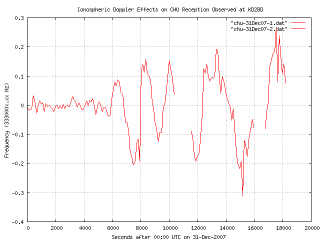
In this plot, the atomically controlled carrier frequency of radio station CHU in Ottawa, Canada was measured and plotted as a function of time, with each reading averaged over a 100 second integration period. While the frequency of the received carrier was fairly accurate and stable for about an hour and a half into this study, a low-frequency oscillation, believed to be the effect of Magnetohydrodynamic waves, developed at the 6000 second point, and grew increasingly intense throughout the measurement period.
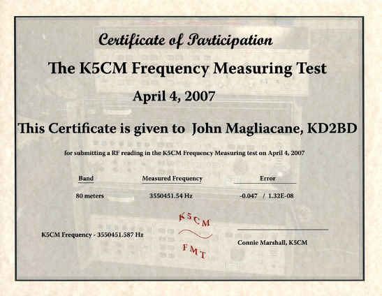
There are two gaps in this plot. The first occurred because data gathering was suspended briefly to participate in a K5CM-sponsored Frequency Measuring Test (where my 80-meter reading turned out to be 0.078 Hz low). The second gap occurred because the test arrangement was left unattended for a period of time, and the VFO drifted to the point of losing phase lock with CHU's carrier. Despite these brief gaps in data collection, the cyclicity is unmistakable.
Doppler shift can be used to determine the effective velocity between a transmitter and receiver in the following manner:
Velocity = (Doppler Shift / Transmitted Frequency) x Speed of Light
Picking a convenient data point, CHU's carrier was found to be approximately 0.15 Hz high at 10000 seconds into the data collection period. Plugging some numbers into the above equation we find the velocity between the transmitter and receiver to be:
Velocity = (0.15 Hz / 3330000 Hz) x 3x10e8 meters per second = 13.5 meters per second
or about 30.2 miles per hour. Since the Doppler shift was positive, if we assume CHU's signal arrived at the receiver in one hop (and the transmitting and receiving sites are stationary), then the height of the reflective layer was decreasing by half this amount, or about 15 miles per hour.
The situation is far more complex than this, but it is an interesting exercise, nonetheless, to try to visualize the undulations taking place in the ionosphere at the time of this study.
Another experiment was performed to discover what effect, if any, antenna polarization might have on the Doppler shifts observed.
During this test, the carrier frequency of radio station CHU was measured using a 0.08 wavelength vertically polarized resonant loop antenna, as well as a half-wavelength horizontally polarized dipole antenna, with the understanding that CHU transmits using vertical polarization.
Since it was impossible to make frequency measurements through both antennas simultaneously using a single receiver and frequency counter combination, a logic control signal was extracted from the frequency counter and used to drive a relay that alternately toggled the receiver between each antenna after making each frequency measurement. The following plots attempt to illustrate how received frequency accuracy was influenced by antenna polarization.
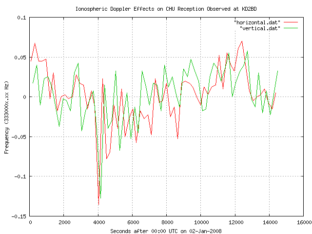
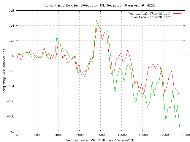
There were times when the frequency measurements were very similar, and others when they were quite different. Most of the time the Doppler Shift trended toward the same direction, but this was not always the case. Faraday rotation taking place in the ionosphere is believed to be responsible for these effects.
One striking observation made throughout this experiment that is not evident in the frequency measurement data is that the signal received from CHU experienced far greater signal fading during horizontal dipole reception times than what was observed using vertical polarization. In fact, it was clearly apparent which antenna was being used during the course of this experiment simply by observing the aural quality of the signal being received at the time.
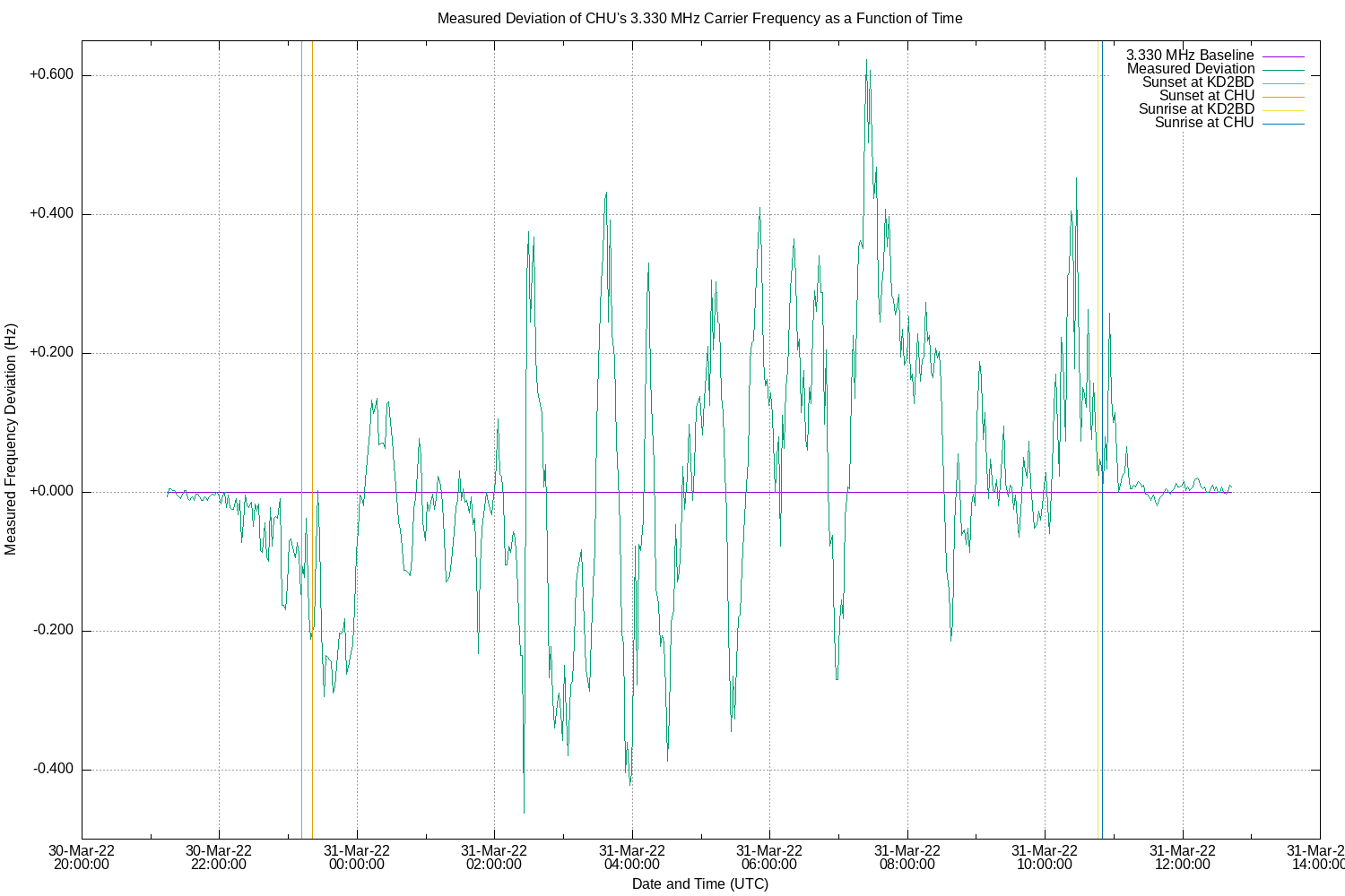
Here is an overnight plot of CHU reception illustrating the effects of sunset, sunrise, and a "Cannibal CME" that struck the Earth's magnetic field on March 31, 2022 at 0210 UTC where it sparked a G1-class geomagnetic storm including visible auroras in some areas.
Short-term propagation effects can be fascinating to study as well. As the following video clip reveals, plotting WWV's 5 MHz carrier against a local standard produces a Lissajous pattern that illustrates some interesting short-term effects ionospheric propagation has on the amplitude, frequency, and phase of the received carrier. Note that on several occasions, while the signal strength remains fairly strong, the phase of the carrier reverses quite abruptly. Meanwhile, there are other short intervals during the sampling period where the amplitude of the carrier becomes noticeably enhanced with reference to the overall average:
The next clip examines reception of radio station CHU on 3.330 MHz by plotting CHU's audio against a local 1000 Hz sinusoidal reference to produce a Lissajous pattern:
We would expect to see the 1000 Hz tone bursts from CHU produce a stationary pattern if the received frequency of the tones measured exactly 1000 Hz. Instead, what we see is a slowly rotating ellipse, especially in and around the time of deep signal fades. This rotation is indicative of a shift in phase between CHU's carrier and upper sideband that is taking place over time. A change in phase over time implies that a change in frequency is also taking place.
CHU transmits using single (upper) sideband modulation with full carrier. Since the audio recovered from the receiver is a product of the received carrier and upper sideband frequencies, the data presented here implies that the carrier and upper sideband are undergoing separate and distinct changes in path length, Doppler shift, polarization, and/or multipath propagation effects, even though they originate from a common transmitter and antenna system, and are separated in RF spectrum by only 1000 Hz (27 millimeters in wavelength).
Dual adjacent carrier FMT transmissions conducted by Connie, K5CM, have permitted further investigation of short-term Doppler effects. The following video clip illustrates AM demodulated audio plotted as a function of time for a pair of 20-meter RF carriers spaced exactly 2000.277 Hz apart. Some very interesting (and yet unexplained) cyclic phase shifts are clearly evident in the following video:
This transmission was received over a distance of 1200 miles by KD2BD in New Jersey using a receiver whose AM detector was used to heterodyne the two carriers together, thereby producing an audio tone equal to the frequency difference between the individual RF carrier frequencies. The resulting audio tone was filtered to a bandwidth of 10 Hz, and plotted against a local frequency standard.
A subsequent transmission that took place on May 20, 2012 under less favorable propagation conditions, revealed more dramatic differential phase shifts between the individual RF carriers:
Despite the less favorable propagation conditions, my submitted frequency measurement for the May 20, 2012 FMT was in error by less than 0.001 Hz!
While the waveforms depicted here appear to "lock in" to a default horizontal position over time and give the appearance of being plotted against a triggered horizontal sweep, the local frequency standard used as a horizontal sweep was not referenced to the instantaneous frequency or phase of the received signal in any way.
The total solar eclipse that swept across the continental United States on August 21, 2017 provided a unique and rare opportunity to study the effects the eclipse might have on radio propagation. Details on an LF radio propagation experiment I conducted during the 2017 eclipse can be found here.
Research, experimentation, and discovery in these fascinating areas of metrology and RF propagation are active and on-going. Further information related to FMT topics can be found through the following links:


No animals were harmed, nor any Micro$oft products used in the creation or distribution of this page.

|
John Magliacane Amateur Radio Operator: KD2BD Open Source Software Developer Internet Advocate Since 1987 Linux Advocate Since 1994 |