Trans Equatorial Propagation in South Africa

Ian Roberts ZS6BTE, December 2012

This article was published in Radio ZS, February 2013

Solar cycle 24 is due to peak in 2013 but “we'll see a very weak solar maximum in 2013, if at all…this could be the last solar maximum we'll see for a few decades.” If you are interested in VHF DX get going – time is running out!

The nature of TEP

Ray Cracknell, ZE2JV (SK) working out of Salisbury, Rhodesia, wrote a fascinating article Transequatorial Propagation of V.H.F. signals in QST Dec 1959. He concluded: - “For the purposes of this account, TE propagation is defined as v.h.f. propagation between points on opposite sides of the geomagnetic equator, and at least 1000 miles from it, without intermediate reflection from the surface of the earth”. It was established during tests with amateurs in 1957-58, particularly in Cyprus, there were two target zones. In the south, from approximately Pretoria (Johannesburg is just south of this zone) up to a line across Africa cutting through northern Mozambique, central Zambia and central Angola. In the north, this main zone commences at the southern Mediterranean and ends in a line through northern Italy across Europe. Extension zones for weaker TEP working encompass a much larger area centred on these zones.

More than 50 years later VHF amateurs in South Africa will agree with these facts. We know the mode is totally dependent on high solar radiation of the F layer.

The ionization centre is the geomagnetic equator sloping slightly southwards east to west from the Horn of Africa to Equatorial Guinea, whereas the geographical equator extends across Africa through the northern tip of Lake Victoria, some 1000 km further south.

It might be a surprise to learn that a transmission from the better sited northern ZS area travels nearly 7000 km before making landfall in the Mediterranean, or further, up to about 8000 km (Austria, Hungary) if conditions are better. Therefore it is not possible to work countries over the greater part of the African continent under typical TEP conditions and logging these countries is challenging for ZS ops.

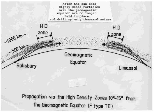
Fig 1: TEP geometry after ZE2JV

ZE2JV noted on 50 MHz a few Watts of power into a simple vertical antenna was received strongly in the northern hemisphere, indicating a path transmission mechanism nearly lossless and resembling a waveguide. From Salisbury he also raised a 432 MHz Yagi to 45 deg elevation and there was no apparent reduction in signal strength received in the Mediterranean area. In cycle 19 (~1958), when these tests were undertaken, the Solar Flux Index peaked at 345 – very high.

According to TV DXer Roger Bunney in his booklet Long Distance Television 1976, at sunset the two daytime F layers break up and merge into the F2 layer approximately 250 miles (400 km) high. This breaks up into small clouds and multiple reflections occur as signals are scattered through the cloud region. Signals, as for conventional F2 layer propagation, suffer multiple images, smearing and have a characteristic flutter effect. In winter the cloud is less expanded by heat and the ions thus more compacted in unit volume, increasing the MUF.

During solar cycle 21, Costas (SV1DH) and ZS6PW (SK) conducted timing pulse tests to learn more about the TEP path using the frequency and time references available at the time. SV1DH writes “Back on cycle 21 (1982), we conducted E-TEP propagation delay measurements from Athens to Pretoria on 28, 50, 144 MHz. The net result was that prop was through depletion ion layer waveguiding at an average height of  600 km, when, after sunset on ionospheric height, this huge irregularity rose slowly hundreds of km and enough to be seen at both ends of path.”

Solar activity peaks every 11 years and the peak lasts 2-3 years. The peak months are around the equinox with the sun over the equator, i.e. March and September. The worst period for ZS is December and January even during active solar conditions when the sun is far south and a long way from the geomagnetic equator. During our mid-winter TEP coupling to Sporadic E in the northern hemisphere, where it is summer, helps the propagation to northern Europe. Sporadic E occurs infrequently in Southern Africa (South Africa has the world’s lowest occurrence) so TEP is easy to identify, unlike other circuits such as N/America to S/America and Australia to Japan which have a high incidence of SpE, so there is room for confusing n/s path SpE as TEP in those areas.

It was noticed in traveling around, operating portable from various locations in southern Africa, there is a TEP gain slope of about 10 dB per 100 km as one travels from Johannesburg northwards towards the northern Limpopo province (Polokwane/Pietersburg). So Polokwane ~300 km north is about 30 dB better off than Johannesburg, for example. As one approaches the Zambezi the gain slope is less steep, but locations such as the Caprivi Strip in Namibia, northern Botswana and northern Zimbabwe are vastly superior locations than anywhere in ZS.

TEP Modes

From the above, TEP is obviously a complex mechanism and in modern terminology has two main modes, to which a sub-mode may be added.

Afternoon TEP (aTEP)

Under current solar cycle 24 conditions (rather poor), from about midday the MUF reaches 48 MHz and TV TXs from Iran, Syria and UAE begin to appear. As the MUF rises further the channel R1 TV TXs on 49 MHz appear from Armenia, Hungary and the Ukraine, etc, followed by 50 MHz amateur traffic such as 50 MHz beacons from the Med (SV1SIX and 5B4CY prominent) and amateur ops from the region.

This mode lasts until after sunset and provides the best DX conditions. The amplitude flutter effect is limited compared to eTEP and there is little frequency shifting of a RF carrier. The frequency stability was confirmed over years by monitoring the German, Swiss, and Austrian 48.25 and 49.75 MHz TV carrier frequencies (now QRT) which were locked to rubidium quality oscillators and generally frequencies were within 1 Hz or so of the nominal value. In other words, there is little Doppler shifting of the carrier, the Doppler “look angle” is also just about zero because of the great distance. This mode may fade out slowly, or transform over the next period to eTEP, typically after about 7.00pm local time.

It would be easy to confuse aTEP with F2 propagation. The difference is the propagation distance. If it were F2, TV carriers, etc from central Africa would be received in ZS. Since they are seldom received during daytime hours, it is easy to ID the mode as aTEP. Day time reception of these TXs would indicate F2 layer operation rather than aTEP.

Fig 2 illustrates multipath as viewed on a TV picture. A TV line scan takes 64 µs, several ghostly images of inverted phase (white instead of black) are visible each side of the main picture information and at the speed of light, 0.3 km per µs, one can calculate the respective times of arrival and glean some information regarding timing of the various picture elements.

It is apparent multipath picture information of the announcer’s face arrives at the beginning and end of a scan line representing distance differences of 0 to 64 µs, i.e. 64 x .3km = 19.2 km and this is maintained for the update rate of 25 Hz (0.04 seconds). It would be interesting to lengthen the scan time if possible to several hundred µs to see just how far in time this multipath exists. Under eTEP propagation (described below) the picture breaks up completely into vertical bands.

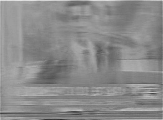
Fig 2: Muro, Portugal on 48.242 MHz received under good aTEP conditions 2.00pm 15 Nov 2011

Evening TEP (eTEP)

Occasionally there would be no aTEP and conditions manifest as straight eTEP after dark. This always indicates poor TEP conditions.

Usually aTEP would change to eTEP with or without a fade-out during the transition and this mode is strongest around 7.30 to 8.30pm or so local time. It provides by far the highest MUF, over 144 MHz from Pretoria and Johannesburg under best conditions and is characterized by “flutter-fading”. TV carriers on 55.25 and 62.25 MHz appear from Syria and Jordan and the TEP path tends to shorten a bit, losing central Europe somewhat and centering on the Med area.

This cycle ZS6 ops have worked to Greece and Italy on 70 MHz from as far south as Johannesburg on CW and WSJT ISCAT modes (SSB in northern ZS) under eTEP conditions. The MUF has peaked about 77 MHz seen from Johannesburg.

The tumultuous nature of the propagation is even more diverse than one would think and this is readily observed on TV pictures received. All synchronization information is destroyed and it is impossible to lock a DX TV picture on eTEP. To counter this a method of turning off sync processing in the Philips demodulation chip in PC TV cards is used so that the picture is displayed stripped of sync (i.e. with a manually adjusted free running time base). Of course the in-band selective flutter-fading caused by multipath reception (group delay) cannot be compensated for and the picture takes on a characteristic appearance reminiscent of water boiling in a pot with fast out-of-context transitions from black to peak white caused by all the phase cancellation and phase summation and placing video AGC processing under pressure.

This multipath has implications for SSB operation and at times copy is difficult with cranky squeaks accompanying drop-out of audio information. CW should not be sent too fast as complete “dahs” and “dits” will be lost, losing the copy. In Fig 3 captured in the time domain, there are frequent dips to noise level in the slow CW caused by lack of reflection and anti-phase combination. And various enhancements, well above the average carrier level, resulting from in-phase combination. Due to all this, eTEP signals might need a higher signal-to-noise ratio to copy them properly. The average signal-to-noise ratio shown is about 10 dB with peaks around 15 dB. The ZS6DN beacon used 4 long Yagis pointed north and 100W apparently.

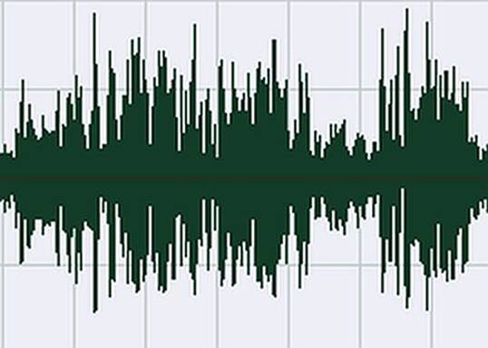
Fig 3: Morse letter “N” from a sound recording by SV1DH in Athens of the ZS6DN 144 MHz beacon 1978.

Sound file processed for display by ZS6BTE

Late Evening TEP (leTEP)

This mode has not been described in any easy-to-read literature I can find. It occurs often enough (possibly around 10-20% of the occurrence of eTEP) in the evenings after 8.00pm, peaks around 9.00pm and may last until 10.00pm local time before slowly fading. It always follows eTEP. It is characterized by a dramatic shortening of the earlier eTEP path, to the extent the Mediterranean region is received very weakly, if at all. It offers VHF communications with central Africa, distance only 3000 km, which flies in the face of conventional TEP mode and distance theory. It does not normally offer an enhanced MUF, and may be limited to 48 MHz or so. Very strong signals are received from the 48 MHz TV TXs in Kenya (particularly), Cameroon and Equatorial Guinea (i.e. across a broad front), and 50 MHz beacons from the area may become audible. Severe multipath and considerable Doppler frequency shift are inherent. It is not sporadic E.

In Fig 4 a “peak hold” function of a few seconds on a spectrum analyzer was used to capture the peak-to-peak Doppler shift of 26 Hz on the Kenya channel E2 TV transmission. The nominal carrier frequency at the time was 48.249961 MHz. It needs a reflecting surface moving at high speed either laterally or vertically or both to produce an effect such as this as the “look angle” is close to zero degrees. Not visible here is the simultaneous (instant) Doppler shift in real time which had both negative and positive values. Kenya is 1000 km south of the normal geomagnetic equator and reception of this TX in ZS indicates the reflecting zone has extended far to the south, so that the TX is “under” the zone sufficiently to allow reflection to the south without exceeding the critical frequency. Latitudinal enlargement of the geomagnetic equatorial zone under good TEP conditions is well documented.

Alternatively, an immense vertical zone of ionization might occur over the geomagnetic equator partially isolating ZS from the northern hemisphere and allowing ready reception of the central African area by back-scatter from this sheet of ionization. This requires intense ionization and compaction of the zone otherwise the critical frequency would be exceeded, yielding only weak back-scatter signals in the south. If this latter possibility is in play, it needs high velocities of reflecting components to produce the measured Doppler shifts illustrated in Fig 4. The vertical sheet possibility becomes attractive when examining amateur stations received under these conditions – African stations on or just south of the geomagnetic equator (Equatorial Guinea, Gabon, Cameroon, etc) are readily received, while stations just north of it (Senegal, Chad, etc), and further north, remain illusive under leTEP.

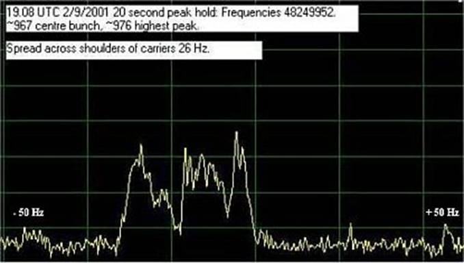
Fig 4: Peak-to-peak Doppler shift of 26 Hz on the Kenya 48.25 MHz TV signal

The frequency shifting phenomenon requires the bistatic range L in Fig 5 to change at a rate fast enough to generate measurable Doppler shift. Bistatic Doppler shift is proportional to the rate of change of bistatic range in period “t1-

t” seconds. Thus, two bistatic ranges are calculated, firstly at time “t”, then at time “t1” seconds. During this time period the target has moved and increased or decreased the bistatic range. The two values are subtracted to provide the change in bistatic range as at time t1.

Change in bistatic range: ΔR = (RTX RRX – L)t – (RTX RRX – L)t1

If the range has increased the Doppler shift will be negative, and positive if the range has decreased. The shift can be negative even if the “target” (the ionized zone) is moving closer to RX. As shown in Fig 4 both shifts can happen at the same time indicating different ionized zones moving at different speeds and directions as viewed by the receiver. Around the ellipse bistatic range does not change or when the target moves along L, so bistatic Doppler shift then is = 0.

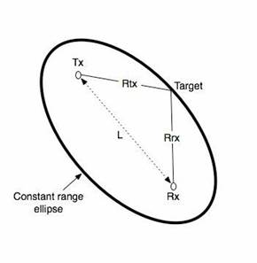
Fig 5: Doppler shift is explained by changes in the bistatic range L (Wikipedia)

TEP backscatter

This works when both antennas point to the north. Intense ionization of the TEP zone is required, such as occurs under ideal eTEP or late evening TEP conditions. Amateur backscattered signals are weak and may not be readable from the Johannesburg area. The situation improves as one moves north along the gain slope mentioned. In the absence of sporadic E in this part of the world it is the way to work on low VHF, other than by meteor scatter, our neighbouring countries.

Equatorial Zone propagation

This mode is an east-west phenomenon and in my experience takes place in the local day time hours commencing at 7.00am, up to dark. Intense solar activity is a prerequisite and the mode is rare in South Africa.

It accounts for a few 50 MHz contacts with Hong Kong, Hawaii and northern Australia. DX entities need to be close to the equator, ~20 degrees, and reception is limited to the northern part of ZS6. It is mentioned alongside TEP as there is the possibility of coupling between this mode and true TEP - Equatorial Zone propagation can circumnavigate the globe all along the equator, or at a small angle to it. It touches down sparingly so there are no propagation indicators and is the longest distance ionospheric mode available on VHF. It is astonishing, for example, to work KH7 (~19250 km) in SSB at 7.00am local time direct path to the east just after equinox (early April 2000) with nothing else heard at the time.

Propagation Indicators

Ops new to 50 MHz, this is understandable, and many experienced ops, can be clueless regarding the many indicators available. For instance, the importance of IDing and using TV transmissions as indicators is relatively new to most amateurs. But the whole of Europe other than Hungary and extreme E/Europe is now QRT on low VHF TV broadcasting resulting from the move to digital TV, so this valuable resource is no longer available. Australia is also QRT on low VHF TV as is the USA and Canada. The oscillators used in the TV TXs listed below are mature, other than the new ones, and don’t change much during 12 years of monitoring.

Table 1: A few important VHF propagation indicators for ZS ops

Item	Frequency	Information – use USB to hear properly
Woodpecker RADAR	34.262 + 15 others!	Southern Russia 7.5 Hz PRF Russian early warning
RADAR	36.924	Cyprus, ionospheric sounding
SNOTEL RADAR	41.700	Nepal snow telemetry, fast woodpecker 14.5 Hz PRF
RADAR	41.424	Cyprus, ionospheric sounding
Cameroon TV	48.249	Central-south, broadband hash no AM sidebands
Kenyan TV 15 kW	48.249952-978	South west Kenya on Lake Victoria – main indicator
Ukrainian TV 50 kW	49.739594	Buky (central) and Simferopol (far south) 1 Hz separation
Russian TV 200 kW	49.747383-411	Moscow
Moldavian TV 12 kW	49.748812-9.749	Cahul
Tajikistan TV 30 kW	49.749987-91	Dushanbe, s/w near Afghanistan border – main indicator
Belarus TV 25 kW	49.750000	Minsk in central Belarus, stable carrier (many TXs at QRG)
Armenian TV 45 kW	49.760420-423	Amasia
SV1SIX beacon 25 W	50.040	Athens, Greece – main indicator
5B4CY beacon 20 W	50.0185	Cyprus – main indicator
VK6RSX beacon 50 W	50.304	Western Australia

This Table has been updated 15 May 2014

There are dozens of 50 MHz beacons listed on the i-net and it’s a good idea to enter some into scan memory, particularly for countries where low VHF TV is now longer in use.

More on TEP

Satellite technology has considerably enhanced our knowledge of the TEP mechanism, referred to in scientific circles as equatorial plasma bubbles, plumes or Equatorial Spread F (ESF) at heights around 400 km. Gravity waves at low latitudes are thought to act as seeds for equatorial plasma bubble formation. Various satellites have been used including military and the GPS range and their beacons are monitored for amplitude and frequency scintillations. Equatorial plasma bubbles are intervals of depleted and irregular plasma densities that degrade communication signals i.e. exactly what is wanted for successful TEP operation from the amateur standpoint. By measuring wave propagation through these plasma bubbles, movements and densities can be derived and used in explanatory modeling. In Fig 6 it is clear the vertical plasma velocity is around 45 m/s (162 km/h) at 20.00 hours (the peak time for eTEP) at equinox March and September. In other words, the plasma bubble has about two hours in the period from sunset to 8.00 pm local time to get to maximum altitude of ~400-600 km depending on the F layer altitude at sunset. For a while after local sunset the layers at attitudes around 400-600 km are still in sunlight and experiencing radiation. When no longer in sunlight the rate of ascent reaches zero around 22.00 hours and goes strongly negative loosing height fast as midnight approaches. The vertical movement is coupled to a predominately eastward movement of the plasma bubble, around 100 m/s (360 km/h); due to local electric fields it is thought. The vertical plasma velocity for strong ESF can reach 50-60 m/s (216 km/h) at a solar flux index of 250 (high solar radiation – solar maximum), falling to 5-10 m/s for a solar flux index of 70 (quiet solar conditions – solar minimum). Thus good TEP conditions require ESF to attain maximum altitude under high solar radiation, and altitude is a more important parameter than the vertical velocity which could be short-lived.

These high horizontal and vertical velocities of the plasma bubble explain the Doppler frequency shifts measured in Fig 4.

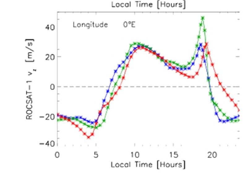
Fig 6: Local time variation of the equatorial vertical plasma drift at longitude 0°E as predicted by the ROCSAT-1 plasma drift model for December solstice (blue), equinox (green), and June solstice (red) for a solar flux level of F10.7 = 150 (Illustration from Stolle, Lühr, Fejer, 2008 in reference section)

Future Solar Cycles

In the references below is a link to an opinion and model concerning solar cycles 24 through 25-26, etc.

At the time of writing this model is proving depressingly accurate. Don’t move QTH in the hope of working great TEP this solar cycle or in the next few..

So far cycle 24 looks likely to top out in 2013 about SFI 180 at best or well down on the last cycle, 23 (SFI 273), which was disappointing enough. By comparison, cycle 21 in 1982 topped out at SFI 290. ZS ops hoping to achieve 100 DX entities on 50 MHz in cycle 24 are in for a hard time and the next cycles are not predicted to add much to the tally and may be restricted to n-s operation to the Mediterranean area, if at all. The decreasing level of solar activity from cycle 21-24 can be seen at http://www.solen.info/solar/images/comparison_recent_cycles.png

Maximum Solar Activity Projection

The sun is in a strange mode regarding solar radiation. Currently only one face is partially active, the opposite face is largely inactive. This causes the 10.7cm Solar Flux Index to alternate with each face between an average of ~145 and only 95 with little variation. The trend is readily displayed at http://www.solen.info/solar/ and has occurred for the last 11 solar rotations and there is no reason to expect changes and it impacts directly on TEP working. From this the table below has been compiled for another 8 solar rotations to June 2013 using the synodic rotation period of 26.24 days (same solar face visible). It looks as though early April 2013 (just after equinox) will produce peak TEP conditions of cycle 24 for ZS ops.

Table 2: Date centres for SFI maxima to June 2013.

Date	Anticipated average SFI peak value
11/12/2012	145
07/01/2013	145
02/02/2013	145
28/02/2013	145
27/03/2013	145
22/04/2013	145
18/05/2013	145
13/06/2013	145

References

Transequatorial Propagation of V.H.F. signals ZE2JV QST Dec 1959 copy at http://www.dxmaps.com/docs/qst_te_dec_1959.pdf

Major Drop In Solar Activity Predicted by Staff Writers Boulder CO (SPX) Jun 15, 2011: http://www.spacedaily.com/reports/Major_Drop_In_Solar_Activity_Predicted_999.html

Long Distance Television Roger Bunney 1976

Relation between the occurrence rate of ESF and the equatorial vertical plasma drift velocity at sunset derived from global observations Stolle, Lühr, Fejer Dec 2008 www.ann-geophysics.net/26/3979/2008/

Solar Terrestrial Activity Report http://www.solen.info/solar/

Bistatic range: http://en.wikipedia.org/wiki/Bistatic_range