Precision Carrier Doppler Analysis
Introduction
With a suitably stable transmission to monitor, and an equally stable SSB receiver, it is possible to measure very tiny frequency
shifts in the received signal frequency that result from changes in the ionosphere. These changes occur because the propagation path
is never static, and in some locations (especially near the poles) and some times of day, the apparent height at which signals are
reflected changes quite markedly, leading to quite easily observable frequency shifts. It is the rate of change of apparent height
which is related to the frequency shift.
In addition, by monitoring a transmission over a long period of time (say 24 hours) you can also measure the signal strength, discover times of day when no propagation exists, and also determine when reception is focussed (direct or by stable refraction) or
diffused (scatter, unstable refraction).
The secret weapon used for this analysis technique is the Narrow-Band Spectrogram. The Doppler shift which occurs generally does not exceed 1 part in 106 (1Hz per MHz), so the spectrogram used needs to have a span of 10Hz or better, and a resolution of better than 0.1Hz to be useful.
VK2BLR received by ZL1BPU Feb 2004
(Click on image for full-sized view)
The spectrogram is a graphical software technique (usually using PC sound card and Fast Fourier Transform Digital Signal Processing software) which allows the user to observe frequency on one axis, time on the other, and signal strength as brightness. In the image above, the horizontal axis is local time (hours), and the vertical axis is frequency (Hz), with a total vertical width (span) of 10Hz. The resolution of the software at the setting used is 256 samples over 10Hz or about 0.04Hz.
Look closely at the image above (click on it for an expended view). This is a recording of reception of a 2W transmission on 3600kHz from VK2BLR, received 2500km to the south-east
of the transmitter. Even during daylight hours (1800 - 2100 local time) the signal was clearly detectable - not what most experienced Amateurs would expect, since during the day the D layer supposedly absorbs the signal before it reaches the ionosphere. However, the absorbtion is not always complete, and the sensitivity of the spectrogram technique allows even a puny 2W signal to be detected via its E-layer daytime reflection. The E layer is relatively stable, and shows little Doppler shift on the scale observed here.
At about 2100 the D layer stops absorbing completely, and the signal starts to be seen from various unfocussed scatter paths, and then reflected from the F-layer. At this time the effective height of the F layer is rising as ion density decreases (now after sunset midway between transmitter and receiver), and as the height increases the reflected signal is low in frequency by several Hz. There are short duration individual paths observed (the more defined dark areas), but much of the propagation is scattered due to the instability of the F layer - no one fixed reflective point, but many reflective points of short duration.
A superb Spectrogram of an Amateur transmission on 3600kHz
In this next picture, the transmission was from the south of the receiver, and the path only 150km, although still outside ground wave range. The late afternoon starts with E-layer propagation and is followed by evening NVIS F-layer propagation. From 1300 to 1600, propagation is moderate strength via the E layer. Variations in frequency here are more likely to be caused by "gravity waves", rather than ionization changes. The relatively low E layer is ionized and de-ionized quite slowly, and so is relatively stable, but the ion density changes as the atmosphere is compressed as the upper atmosphere heaves up and down, in effect causing small short duration cyclic changes in barometric pressure at the lower altitude E-layer reflective point. Between 1600 and 1700 a second effect becomes clearly visible. The recording was made in winter, and the attenuating D layer dies away early, now allowing F-layer returns to be detected, and both E- and F-layer paths are visible.
At about 1730 the E-layer signal fades out (in all probability it is now simply swamped in the receiver by the AGC action of the much stronger F-layer signal), and scatter is also now noticeable. The apparent downward frequency shift is because the F-layer reflective region is rising as the ion density drops after sunset. The F layer is strongly affected by the earth's magnetic field, and the ions spin in ellipses rather than circles, with the result that the refractive index is different for waves of different polarizations. Thus there are two reflected signals visible (especially clear from 1900 - 2000). These are the O and E rays (Ordinary and Extraordinary), although it is not possible to tell which is which. Scatter is also stronger and quite clearly lower in frequency. From time to time as the evening progresses, focussed areas of signal appear in the scatter, probably due to multiple reflections from the earth and ionosphere. Late in the evening the F layer active region reaches stable ion density and the Doppler shift is reduced.
The straight line above the received signal is an artifact in the receiver, but serves to show the AGC action - when this trace is weak, the ionospheric signal is strong.
NVIS Spectrogram of an Amateur transmission on 3840kHz
This third picture is of a transmission only 10km from the receiver. As a result the ground wave signal is present all the time.
The transmitter had only 2W output. This is a classic example of NVIS propagation, and was recorded during the very early morning. At the left, the F-layer return is slightly above frequency, and is becoming weaker as time progresses. At about 0330 it splits into O and E rays, and the two die out at quite different times, 30 minutes apart! There is then no visible propagation (apart from ground wave) from 0430 until 0630, when the sun reactivates the F layer. The implication is that the MUF has dropped below 3.8MHz, so the ionosphere is no longer supporting near vertical reflections (it would probably still reflect oblique signals).
When the F-layer signal returns with sunrise, the F-layer ion density is increasing and the apparent reflection height lowers, causing an up-shift in the returned frequency. Note how between 0630 and 0700 there appears to be another, but less defined, 'echo' above the main F-layer return. This extra return has exactly twice the Doppler shift, which indicates that it is caused by double reflection from the ionosphere (up, down to earth, back up and down again). Triple reflections are not uncommon. After 0730 the F layer signal dies away as the D layer begins to attenuate the signal going up and again coming down. Because the D layer is the lowest, it is the slowest to ionize.
The vertical marks every 10 minutes on this image are caused by periodic CWID on the transmission, and the fuzz close to the carrier is caused by transmitter synthesizer noise. This little transmitter is locked to TV sync and achieves 1 part in 108 carrier accuracy. Note that the ground wave signal is dead straight. The complete lack of drift on the recording, which is only 2.5Hz wide, is because the receiver also achieves better than 1 part in 109 stability. (It is locked to a Rubidium Standard).
Many other propagation conditions can be analysed in this way, but the reflective height or time-of-flight of signals cannot be measured with this technique. Analysis is best supported by studies of propagation using other techniques.
Suitable Transmitters
To be useful for this technique, the transmitter must be very stable (preferably the stability should be better than the receiver resolution), which means one part in 107 or better. Few Amateur transmitters meet this requirement! High power is not required, even if very long paths are contemplated. Standard Frequency stations such as WWV are ideal, and some HF broadcast stations are also useful, except that they are rarely on the same frequency for more than a few hours at a time. Most other HF transmissions are simply not stable enough! Of course for Amateur band measurements, you will need either a homebrew special-purpose transmitter, or use a
commercial signal generator or exciter with a high stability reference.
Many professional signal generators have sufficient stability and output power, and can be externally locked.
The FEI FE-5650A and FE-5680A Rubidium Synthesizers make excellent signal sources. The author uses a
Redifon DU-505 Synthesized Drive Unit (ISB exciter, 6.4MHz OCXO, PLL synthesizer), with a Codan amplifier, locked to the HP Z3801A GPS Reference, and a JRC NMA-73D Exciter (1MHz OCXO reference, PLL synthesizer) with associated JRC CAR-45B amplifier.
It is quite practical to build your own transmitter with the necessary stability. A transmitter designed by ZL1BPU, and used by VK2BLR, ZL3JE and others, is a simple two-chip micro-controlled unit, phase-locked to GPS or TV sync. This unit easily manages 108 stability when locked to a suitable TV sync source. Another interesting and more versatile option would be to build
a DDS VFO using an AD9835 device and a high quality TCXO as the reference.
The little transmitter illustrated below has only one part in 106 stability, but gives quite good results on 80m if kept in a stable environment. It is
inexpensive to build and easy to get going. The TCXO reference is a 2ppm unit from an old cellular phone.
The output is about 500mW, quite sufficient for good Dopplergrams, and the transmitter is efficient,
drawing only 100mA from a 12V supply. See the Technical Description
for more information.
QRP Transmitter for Dopplergram measurements on 80m
(Click on image for full-size drawing)
SUITABLE RECEIVERS
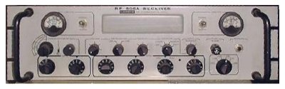

Harris RF-505A Receiver (left) Transworld TW100 (right)
The main requirement of a good receiver for Doppler measurement is stability. Single-reference
commercial, military or marine receivers are generally more stable than conventional multi-crystal synthesized Amateur radios. An oven-controlled or external reference receiver is best. Look for ex-military receivers, higher-spec marine transceivers, and modern single reference Amateur transceivers with a 'high stability' option.
It is also helpful if the receiver has AGC switched off or disabled. It will take plenty of practice to find suitable signals to monitor and to get good results.
Some receivers and transceivers use different band oscillators for each band, and a different oscillator for the BFO on USB from LSB. These receivers will potentially have systematic errors that mean that calibration performed on one band and one sideband will not be transferrable to other bands or BFO settings, and will need to warm up again as you change bands! If the only available receiver has less than perfect stability, warm it up on the correct settings for several hours before making recordings, and keep the shack temperature as constant as possible. Don't even think of using a VFO-controlled radio!.
The author currently uses three high quality receivers:
- A RACAL RA6790/GM (single reference using excellent 1MHz OCXO) which uses PLL synthesis. This radio is locked to an HP Z3815A GPS Disciplined Reference to achieve better than 1 part in 1010 stability.
- A Kenwood TKM-707 (modest single reference OCXO, 1 part in 107) which uses PLL and DDS synthesis.
- A Transworld TW100 (modest single reference OCXO, 1 part in 107) which uses PLL synthesis.
Kenwood TKM-707 Marine Transceiver

RACAL RA6790/GM Receiver
For single frequency use, the Codan 7004 crystal-controlled receiver is quite suitable. Effort put into improvement of receiver stability and accuracy is well worth while, although some receivers are extremely difficult to tame. The author has worked long and hard with an otherwise excellent Icom IC-R71 (multi-crystal PLL synthesizer), and has still not achieved acceptable stability.
SPECTROGRAM SOFTWARE
The Spectrogram is a graphical computer program designed to display frequency on one axis (usually vertical) and time on the other, with the third axis (brightness) indicating signal strength. Most of the programs operate in real time using input digitized from audio by a PC sound card. Some use data from an external digitizing source, such as a DSP unit. The most useful Spectrogram programs also offer an amplitude versus frequency display (spectrum display) and digital signal strength and frequency measurements for the strongest frequency component detected. In this way frequency resolution to 0.01Hz can be measured.
The Spectrogram uses an FFT technique, and the best types for this application use narrow-band low sampling rate with windowing, allowing frequency spans as low as 5Hz or less to be viewed without loss of resolution. The dynamic range of sound cards and FFT software is very good, enabling frequency measurements to be made on weak signals, and comparison of signals of quite difference signal strengths. Some Spectrogram programs are optimized for different purposes (full audio range, high speed, or very weak signals) and are not always as useful for frequency measurement purposes. The programs described below are recommended specifically for their Doppler recording performance.
Spectran
Written by Alberto I2PHD and Vittorio IK2CZL, this is probably the most universally useful program. Used at the lowest available sampling rate and with manual gain adjustment, Spectran does a good job if the gain adjustments are made with care.
For Doppler monitoring, Spectran works very well, although setting brightness and contrast optimally takes some skill and patience. The next image, thanks to Dave ZL1MR, is an example with NVIS O and E rays and backscatter, received on 3840kHz at a range of 15km. The transmission was from ZL1BPU (40mW) and this recording represents about two hours across sunset. The weak slightly curved but stable line is the ground wave, bent by receiver warmup drift. The point where the signal splits into Ordinary and Extraordinary rays from the ionosphere is clearly evident and much stronger that the ground wave, and spectacular clouds of backscatter are also visible. If you look closely you'll also see brief 4Hz sideband dots every 10 minutes. These are caused by the 10WPM Morse ID on the transmission (who says a Morse transmission has no bandwidth?)
ZL1MR's SPECTRAN recording of ZL1BPU on 3840kHz
Spectran is also useful for general signal monitoring and narrow drift measurements. The calibrations on the display are excellent. With the software AGC on, the signals tend to be "washed out", losing detail.
Download Spectran from www.weaksignals.com.

Spectran in Doppler mode
(click on the picture for a closer view of the settings)
For Doppler monitoring, set Spectran at 8000 or 5512 samples/sec and use 0.031Hz resolution or better. Set Auto-brightness (Auto brig.) off, use the low gain setting and keep the Brightness and especially Contrast close to the minumum settings.
Spectrum Laboratory
By Wolfgang Buescher DL4YHF, Spectrum Laboratory is very complex to use, but is very capable for a wide range of applications. To use it well you must understand FFT technology well, and must use a fast computer (over 500MHz preferably), with plenty of memory. It has several advantages, including user-settable presets with offset and gain calibration, and the ability to record amplitude data. The cursor readings are three dimensional - frequency, amplitude, and time. Horizontal and vertical time scales are available. See
the DL4YHF website.
G3PLX Programs
Two excellent programs are offered by Peter G3PLX. The first is EVMSPEC, which uses the Motorola DSP56002EVM development board. This program digitizes the data with an external DSP unit, and send the data to a PC display application via a serial port. There are two particular advantages to this approach - very fine spectrograms with high resolution, and independence from the sound card (which means you can run two spectrograms at the same time on older PCs). SBSPECTRUM for the PC sound card is probably the best program anywhere for PC sound card Doppler measurements. You can easily run multiple instances on a modern Win XP computer. Both programs offer fine
resolution and a narrow 2.5Hz span. Start with settings 1000Hz Centre Frequency, 10Hz span, and slow the Sample Interval down to 20.48 seconds. Set the receiver 1kHz low of the signal to be studied, running USB, preferably with the AGC off or the RF gain backed off.
The SBSpectrum software is only available by applying directly to Peter Martinez.
A typically beautiful EVMSPEC spectrogram (WWV backscatter on 10MHz plus local OCXO Reference)
Copyright � Murray Greenman 1997-2009.
All rights reserved. Contact the author before using any of this material.