|
|
|
Introduction
To define the performance of a receiver or transmitter, various specifications are recorded which are obtained from measurements carried out. Perhaps the least understood of these in amateur radio circles is intermodulation performance and how it is measured. The aim of this article is first to discuss intermodulation products and how they are produced and then look at how they are defined and measured.
What are Intermodulation Products?
When a single frequency (f1) is fed through a device whose output is not a linear function of its input, harmonics of f1 are generated, i.e. 2f1, 3f1, 4f1, 5f1, etc (no device is perfect and so harmonics are always generated even at low levels).
Now, if two separate frequencies exist together in a non-linear device, sum and difference frequencies are also produced in addition to the harmonics. This can be shown mathematically to be the result of a multiplication process between the two original frequencies and hence the two new frequencies are called products. If the two original frequencies are f1, f2 and the highest frequency is f2, then we can expect two other components (or products) of (f1+f2) and (f2-f1). However, it doesn't stop there. Since there are harmonics of f1 and f2, then there will be sum and difference products between all of the harmonics and the fundamentals and between each other. These are the intermodulation products which are frequency components distinct from the harmonic components discussed in the previous paragraph. Of course, if there are more than two fundamental frequencies, then the multitude of products is compounded further.
It can be shown, using a mathematical series, that when harmonics are generated, the harmonies extend upward in frequency to approach infinity, progressively decreasing in amplitude as the frequency increases. Likewise, the intermodulation products could also be considered to be infinite in number. However, we are only really interested in those of practical significance, that is of such a level that they might deteriorate the quality of our signal beyond an acceptable level.
To examine intermodulation products we will consider two frequencies f1 and f2 and some of the orders of intermodulation products. To define the order, we add the harmonic multiplying constants of the two frequencies producing the intermodulation product. For example, (f1+f2) is second order, (2f1-f2) is third order, (3f1-2f) is fifth order, & etc. Let's consider f1 and f2 to be two frequencies of 100 kHz and 101 kHz respectively, that is 1 kHz apart. We now prepare Table 1 showing some of the intermodulation products.

Looking carefully at the table, we see that only the odd order intermodulation products are close to the two fundamental frequencies f1 and f2. One third order product (2f1-f2) is 1 kHz lower in frequency than f1 and another (2f2-f1) I) is 1 kHz above f2. One fifth order product (3f1-2f2) is 2 kHz below f1 and another (3f2-2f1) is 2 kHz above f2. In fact it is the odd order products which are closest to the fundamental frequencies f1 and f2.
Let's expand further the odd order products as shown in Table 2.
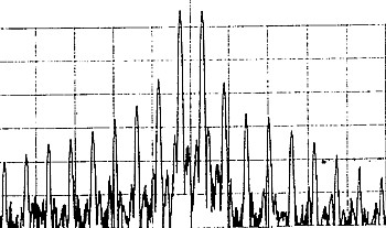
The series of odd order products can be seen to descend and ascend progressively in increments of 1 kHz from the two fundamental frequencies f1 and f2 respectively. A typical spectrum produced could be depicted as shown in the chart of Figure 1.

Of all the harmonics and intermodulation components produced, are often only interested in those which fall in. the passband of our equipment and, in the case of the intermodulation components, those which happen to be closest to our fundamental frequencies. The third order components are the closest and also usually the highest in amplitude. Because of this, they are usually the products of most concern and are those which are commonly measured and defined in transmitter and receiver performance specifications.
Effects of lntermodulation Components
The existence of intermodulation components affects the performance of equipment in various ways. First let's look at audio amplifiers. The presence of any component at the output of an amplifier, but not fed into it, degrades the quality of the signal being amplified. We call this distortion, which can be the result of non-linearity in the amplifier causing the generation of harmonics of the signal frequencies and, in turn, intermodulation components. So we have harmonic distortion and intermodulation distortion which can individually be defined. We often see intermodulation distortion abbreviated to IMD.
Some different effects can be experienced when non-linearity exists at RF in a transmitter and, in particular, in the final linear amplifier of the transmitter. Consider the amplifier delivering sideband components to the antenna at radio frequencies and because of nonlinearity, harmonics of the various sideband components are generated plus various intermodulation, components. The harmonic components and the even order intermodulation components will be well spaced away from the operating frequency, and hopefully attenuated by the tuned amplifier tank circuit and the antenna tuning system. Not so for the odd-order intermodulation components which are closely spaced around the fundamental components from which they were generated. First of all they will show up as audio distortion after being received and detected by the radio receiver. However, that's not all! We have seen from the previous paragraphs that the odd order components spread out either side of the fundamental components in progression gradually decreasing in amplitude. The effect is to broaden the radiated signal and in receiving the signal, we experience the familiar sideband splatter. As most of us well know, this causes interference to others trying to use another channel near in frequency.
Another application where those odd order, intermodulation components are of considerable concern is in the first Mixer stage of a superheterodyne receiver. The special function of the mixer stage is to produce some form of non-linearity so that an intermediate lower frequency is formed from the sum or difference between the incoming RF signal frequency and a local oscillator frequency. The mixer stage is, therefore, a prime spot for other intermodulation products which we might not want. Let's look at an example. Our receiver is tuned to a signal on 1000 kHz but there are also two strong signals, f1 on 1020 kHz and f2 on 1040 kHz. The nearest of these (f1) is 20 kHz away and our sharp intermediate frequency (IF) stage filter of 2.5 kHz bandwidth is quite capable of rejecting this signal. However, the RF stages before the mixer are not so selective and the two signals f1 and f2 are seen at the mixer input, free to produce intermodulation components at will. Now work out the third order intermodulation component (2f1-f2) and we get (2x 10²⁰-1040) = 1000 kHz, right on our signal frequency. This is just one example of how intermodulation components or out-of-band signals can cause interference within the working band.
Another form of interference in receivers which results from the mixing of intermodulation components is Cross Modulation. This becomes more apparent when dealing with AM signals and the modulation on a strong out-of band signal transfers itself across to modulate the signal being received. The process is probably complex but, due to non linearity in the receiver, one can well imagine the carrier and sideband frequencies of the out-of-band modulated signal mixing to produce difference second-order components at the audio frequencies of modulation. Due to the same non-linearity, the unwanted audio components intermodulate the signal being received. If the receiver is designed for good intermodulation immunity, it will also have good cross modulation immunity.
Receiver IMD Performance
To assess the receiver for its tolerance against interference from internally generated intermodulation products, the receiver is tested for its sensitivity to third-order products using two equal level signals fed to its input and typically 20 kHz apart. The receiver is tuned to the frequency of one of the third order products derived from the two signal frequencies. The level of the combined signals at the input is adjusted until the detected output level is equal to that generated by the receiver's self noise. That is, there is a 3 dB change in output level between when the signals are on and when they are off. The level of the third order product necessary to produce output equal to the receiver "noise floor is recorded. For the purposes of following discussion we will call this level IMD Threshold.
We also need to know the normal signal input level which produces audio output equal to that of the receiver's own inherent noise or its noise floor. This is done by tuning the receiver: to one of the two frequencies and again adjusting input level to give an output level 3 dB above the noise output level. For the purposes of the discussion we will record this input level as the Signal Threshold. The difference in dB between the IMD threshold and the signal threshold is called the Intermodulation Dynamic Range or IMD Dynamic Range. The higher the difference, the better the immunity to interference from IMD products.
Now, there is an important characteristic of the third-order products which makes their presence more of a problem than one might first imagine. Assuming no compression (due to AGC, etc), output from a fundamental signal is proportional to input, ie for 10 dB rise in input level there is 10 dB rise in output level. However, the output of the third order product is proportional to the cube of signal input level and, for a 10 dB change in input level, the product increases by 30 dB.
Now refer to Figure 2. One curve plots a linear rise in output level against input level for the fundamental signal frequency. The other plots the level of third-order IMD products against input level, the output rising 30 dB for every 10 dB change in input level. At an output level equal to the noise floor, the two curves are separated by an input level difference equal to the IMD Dynamic Range. As the intermodulation curve rises with greater slope than the fundamental curve, they cross at a point called the Third-Order Intercept Point where the intermodulation product output level is equal to the fundamental signal output level.

The Third-Order Intercept point is normally a theoretical point well above the receiver overload level. However, it is often specified to define intermodulation levels, and particularly in specifications for mixer packages.
The Third-Order Intercept point can be derived on decibel scales by first extending the signal curve linearly from the signal threshold point on the noise floor axis so that output level increase in dB equals input level increase in dB. Mark the IMD threshold point on the noise floor axis. This is at an input level higher than signal threshold by an amount equal to the IMD dynamic range. Mark another point on the noise floor axis beyond the IMD threshold point by an amount equal to half the IMD dynamic range. Extend this point vertically to cross the signal curve and this is the Third-Order Intercept point. Join this point to the IMD threshold point to complete the curves such as is shown in Figure 2. In the diagram, the noise floor input level is -120 dBm, the third order components become detectable at 40 dBm and the IMD dynamic range 80 dB. The theoretical third-order intercept occurs at an input level of 120 dB above the noise floor input level.
It can be seen from the curves of Figure 2 that, above the IMD threshold level, the IMD products can become quite a problem. In the example, IMD products from out-of-band signals at an input level of -40 dBm would barely be apparent. Increase the level by a mere 10 dB and the interference from these products would increase by 30 dB.
Receiver Measuring Gear
To carry out intermodulation performance on a receiver, the set-up shown in Figure 3 is required. The RF outputs of two signal generators are combined in a hybrid circuit designed to prevent interaction between the two generators. A hybrid circuit is balanced so that a signal at any one input port cannot reach the other. However, both signals appear combined at an output port.
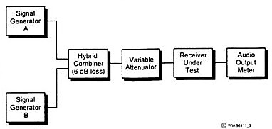
The combined output is fed to the receiver via an adjustable attenuator with a range up to around 80 dB and resolution of 1 dB. Assuming that the receiver has an input resistance of 50 ohms, both the combiner and attenuator are designed for a circuit impedance of 50 ohms.
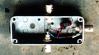
A hybrid combiner and attenuator assembled by the writer is shown in Figure 4. The hybrid circuit, Figure 5, is one taken from the ARRL Handbook. The combiner has an insertion loss of 6 dB for each signal channel.
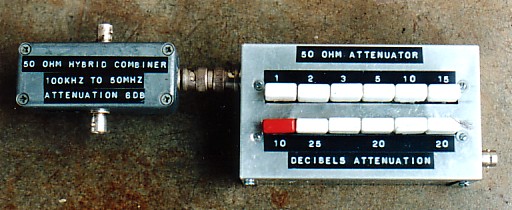
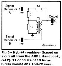
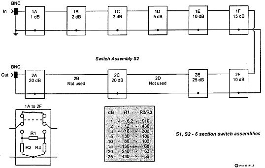
The attenuator was made up using two mechanically interlocking, in-line switch assemblies of the type similar to those used in older style push-button car radios. The assemblies, each of six switches, were recovered from some old intercom units and each switch came with plenty of change/over contacts to switch in or out an attenuation pad. One assembly switches in 1 dB, 2 dB, 3 dB, 5 dB, 10 dB and 15 dB pads. The other switches in 10 dB, two of 20 dB and 25 dB pads. Up to three switches on each assembly can be simultaneously pressed to lock in so that up to six pads can be in circuit together to provide a continuous selection of total attenuation between 1 and 95 dB. The circuit diagram of the complete attenuator is shown in Figure 6.

The only other device necessary is some form of AC voltmeter to measure the comparative level of audio signal at the receiver output. All it is required to do is to record a 3 dB change in level above the receiver noise floor. In terms of voltage increase, this is a rise of 1.4 times.
Our references have so far been made to levels in dBm, or decibels referred to one milliwatt. However, signal generator outputs are commonly calibrated in microvolts and millivolts with scales in multiples of 10. To convert between units, 1uV across 50 ohms is - 107 dBm. Each time the voltage is multiplied by 10, add 20 dB so that 10uv is 87 dBm, 100 uV is -67 dBm, etc.
To find the signal threshold, set one signal generator to a fairly low level (say 10uV or -87 dBm) and tune the receiver to the signal generator frequency. Adjust the attenuator so that the signal raises the audio output signal just 3 dB (1,4 times volts) above the noise level (measured with signal off). The signal threshold in dBm is equal to -87 dBm, minus the loss in dB set by the attenuator, minus 6 dB loss in the hybrid combiner.
To find the third-order IMD threshold, set the two generators (20 kHz apart in frequency) to an equal level somewhat higher, such as 10 mV (-27 dBm). Tune the receiver to the frequency of one of the third-order products. Adjust the attenuator until the audio output from the third-order signal is just 3 dB above the noise level. The IMD threshold is equal to -27 dBm, minus the loss in dB set by the attenuator, minus 6 dB loss in the hybrid combiner.
Transmitter Tests
To check out a single-sideband transmitter for those intermodulation components which cause sideband splatter, we need a two tone audio generator to feed into the microphone input of the transmitter. This can be quite a simple test unit, consisting of two fixed frequency oscillators delivering the same output level into a resistive network which combines the two signals. Simple two tone generators have been presented in Amateur Radio from time to time. In the March 1983 issue, the writer described one using two FX205 Tone Generator packages. In this one, frequencies were set at 1000 Hz and 1600 Hz.
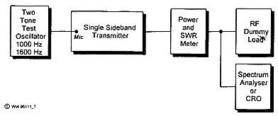
A test arrangement for the transmitter is shown in Figure 7. The two tone oscillator level is adjusted to provide full RF power from the transmitter into a dummy load. Power can be monitored with the usual Power/SWR meter. Apply the audio signal in short bursts as most single-sideband transmitters are designed for speech and the final amplifier stage might be damaged if sustained on continuous full power. The best way to monitor the level of the various intermodulation sideband components is to examine the RF output signal using a Spectrum Analyser.

Figure 8, taken from March 1966 issue of QST, is a typical spectrum analyser display of the RF output of a single-sideband transmitter fed with two audio tones 1000 Hz apart. Two fundamental RF sideband frequencies are created but we can also see a family of odd-order intermodulation frequencies, either side of the two fundamentals with all frequencies spaced 1000 Hz apart. The display shows that the third order products are around 21 dB below the fundamentals, the fifth order 30 dB below, the seventh order 33 dB below, & etc., in decreasing amplitude as the order progresses.
Whilst the spectrum analyser is the order of the day in the modern electronics laboratory, not many radio amateurs could boast of one in the radio shack. However, the Cathode Ray Oscilloscope (CRO) is a more common piece of test gear, and with this we can get some idea of whether there might be an excessive spread of intermodulation sideband components. Figure 9, taken from the ARRL Handbook, shows CRO displays of the RF output generated from a two tone audio source fed to the transmitter. In diagram A, the waveform is quite good and we could expect a fairly clean signal transmitted. In diagram B, compression of the waveform peaks is occurring, possibly because the final amplifier is being driven too hard into a state of poor linearity. If there is poor linearity, then we can expect intermodulation components to be generated and sideband splatter.

Another test that might be applied is to demodulate the transmitter so that we get the two tones back as audio. Perhaps a station receiver can be used for this purpose if it can be prevented from being overloaded by the transmitter. The audio intermodulation distortion tests as described in the following paragraphs can then be carried out. The tests could apply to any mode of transmitter and matching receiver whether it be SSB, AM, or FM (for AM, a simple rectifier and RF filter would be adequate for demodulation). The only problem with this form of test is that the distortion measured is the combined distortion of both transmitter and receiver. If excessive distortion occurred, one would have to be certain that it wasn't caused by the receiver.
Measurement of Intermodulation Distortion at Audio Frequencies
As with other tests described, two audio signals at different frequencies are fed through the device to be tested and the output is monitored. If a modern spectrum analyser is available, the relative amplitudes in decibels from all components at the output can be displayed. As the X axis of the analyser display is calibrated in frequency, the various intermodulation components can be identified and their amplitudes recorded relative to the two fundamental frequencies.
Another instrument of a past era, but which can do a similar job, is the Heterodyne Wave Analyser. This is, in effect, a sharp tuneable filter which achieves its sharpness and tuneability by heterodyning the measured signal with a tuneable oscillator and passing the difference frequency through a sharp fixed 50 kHz crystal filter. By adjusting the tuneable oscillator, the various frequency components can be selectively tuned in and the outputs at 50 kHz can be compared. The Wave Analyser was described in the writer's previous article on Measurement of Distortion, Amateur Radio June 1989.
Another method to measure the intermodulation level is to make use of a CRO display as shown in Figure 10. Two audio signals of widely different frequency are combined and fed into the device under test. The lower frequency signal has an amplitude four times that of the higher frequency signal. The output of the device is fed to the CRO vertical plates via a high pass filter which removes the low frequency signal. The CRO time base is externally synchronised to the low frequency signal. Intermodulation is shown on the display as an amplitude modulation waveform of the lower frequency on the higher frequency carrier. The reason for the four to one signal amplitude ratio is to amplify the apparent modulation and improve resolution in reading the display. The test set-up, shown in Figure 10, uses a 100 Hz low frequency signal and a 2000 Hz high frequency signal. A simple resistive mixing network is used to prevent interaction between the audio generators. Referring to Figure 11, percentage intermodulation is calculated from a and b scaled on the CRO display as: % Intermod = (a-b)/2(a+b) x 100.

In this test, it should be clear that we are essentially measuring the effect of the second-order intermodulation components at (f2-f1) 1900 kHz and (f2+f1) 2100 kHz. This should not be confused with the fact that at radio frequencies we had been mainly concerned with the odd-order products because it was those which appeared in close to our tuned band. However, at audio frequencies, both odd and even products fall within the audio band.

Summary
Intermodulation products have been discussed with particular attention to how their presence affects our transmitter and receiver circuitry. In audio circuits, they are one of the contributing distortion factors which deteriorate audio reproduction quality. At radio frequencies in transmitters, they appear as what we recognise as sideband splatter. In receivers, circuits susceptible to intermodulation encourage interference from signals outside the receiver pass-band.
Various ways have been explained as to how intermodulation components can be measured and how the equipment performance in terms of IMD susceptibility can be specified. The reason why the third order performance is usually defined in RF circuits has also been discussed.
References
1. Lloyd Butler VK5BR: Measurement of Distortion - Amateur Radio, June 1989.
2. ARRL Handbook 1989: Chapter 25 Test Equipment & Measurements; Chapter 18 - Voice Communications.
3. Jon Dyer G40BU.. High Frequency Receiver Design - Radio and Electronics World, July 1983.
4. Lloyd Butler VK5BR: A Discussion on Mixers -Amateur Radio, April 1988.
5. Lloyd Butler VK5BR: Two Tone Test Oscillator for SSB - Amateur Radio, March 1983.