FOREWORD From the author

This article was published in Amateur Radio in 1985. I decided that it was worth retrieving in this year (2010). The described procedure makes use of the "L Match" to load up, against ground, a random piece of wire or antenna made for a higher frequency.

The L match makes use of the characteristic of a resonant tuned circuit in that the parallel resistance across the circuit is equal to the resistance seen in series with it multiplied by (Q + 1) squared. By making the matching circuit resonant in conjunction with the antenna constants and selecting the L and C components to set the Q as required, the resistive component of the antenna is made to appear larger or smaller at the input of the matching circuit. If the antenna resistance component (Ra) is lower than the required load resistance (Rp), usually 50 ohms, then the antenna is connected in series with the tuned circuit and the transmitter line connected in parallel with it. If the antenna resistance component (Ra) is higher than Rp, then the reverse is connected with the antenna across the tuned circuit and the transmitter line connected in series with it. (See also Later Footnote at end of article).

There are two reactive components in an L match, one is in series and one is in parallel. One is an inductor and one is a capacitor. Combined with reactance of the antenna, they form the tuned circuit and their values are selected to achieve the required value of loaded Q. . Whether the shunt or series component comes first depends on whether the reflected resistance is to be made greater or lower than Rp. Which of the L or C components goes in series or parallel depends on choice of design - either can be in either place.

The article makes use of some formulae which have been worked out for the L Match and includes a number of curves to assist in selecting the required values of L and C for 1.8MHz. To reproduce the figures, they had to be photo-copied from an ageing printed copy of amateur Radio, December 1985. Despite some enhancing of the images, their reproduction here is not as good as I would have preferred.

INTRODUCTION

As amateurs, most of us are restricted to an antenna system which must fit into a standard house block. If we venture down to the medium frequency band on 1.8MHz, we are usually restricted to operating with whatever length of wire we can manage, connected with an earth or counterpoise system. Such a system, particularly if the wire is less than an electrical quarter wavelength, leads to a number of problems in coupling to the transmitter.

ANTENNA EFFICIENCY

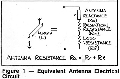
The first problem is one of antenna efficiency. Referring to Figure 1, the antenna resistance (Ra) is the sum of radiation resistance (Rr) and the loss resistance (RL) the antenna system. Loss resistance is the result of a number of factors including leakage loss across insulators, the AC resistance of the antenna conductors and, most significant of all, the earth resistance. Also, not to be overlooked is the additional loss resistance of any loading inductance used in matching to the transmitter.

Antenna efficiency is calculated as follows:

EFFICIENCY = 100 Rr/(RL + Rr) %

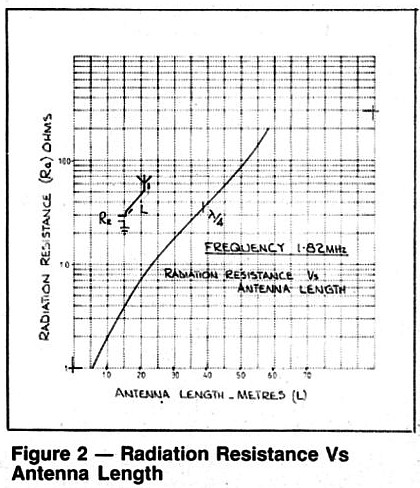
Referring to the curve, Figure 2, radiation resistance falls rapidly as the antenna length is reduced, also reducing efficiency because greater proportion of power is being absorbed in the loss resistance.

If antenna efficiency is to be optimised, the antenna should be as long as possible and earth resistance kept low, particularly if the antenna is shorter than a quarter wavelength. Wired radials, counterpoise or earth mat, are of value in reducing earth resistance.

Loss resistance can be checked by first measuring the antenna constants Ra (antenna resistance) and Xa (antenna reactance) with an impedance bridge. The measurements can be carried out quite well with the familiar noise bridge, used by many amateurs. If the bridge is calibrated directly in reactance at one frequency, do not overlook correction for 1.8MHz.

Now refer to Figure 2 to obtain the nominal radiation resistance (Rr) for the length of antenna in use. Subtract this value from Ra and the result is loss resistance (RL). Antenna efficiency can be now calculated from the previous formula. If antenna efficiency is low, consideration might be given to improving the earth or increasing the antenna length. The constant Xa obtained will be considered later in the text.

ANTENNA MATCHING

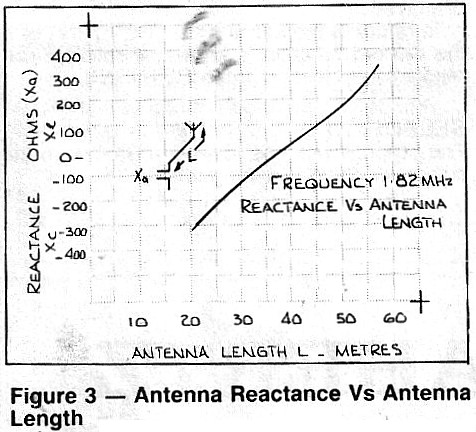
The second problem concerns the correct matching between the transmitter and antenna. Most modern transceivers are designed to operate into a 50 ohm resistive load and do not tolerate much divergence from that impedance. The antenna, however, has resistive and reactive components which vary with length. The resistance component has already been discussed. A typical example of the reactive component (Xa) varying as a function of length is shown in Figure 3.

Attempts to match the antenna to the transmitter using the typical antenna tuning unit (ATU) might not prove successful because of insufficient range in the ATU tuning capacitors. At 1.8MHz, loading capacitance needed could well be in the nano-farad regions, (1nF = 1000pF)


Loading can be better achieved by a network of fixed reactive components selected to form a correct match. To design a network, the antenna resistance (Ra) and the antenna reactance (Xa) must be first measured with the impedance bridge as discussed previously. Now proceed as follows:


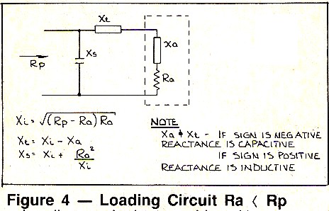
If Ra is less than the desired load resistance (Rp) at the transmitter, use the circuit of Figure 4 and calculate thus:

i. Reactance Xi = √[(Rp - Ra).Ra]

ii. Calculate the series reactance Xt = Xi - Xa

Note that if Xa is capacitive, its sign is negative and therefore its value is added to Xi.
If the resultant Xt is positive, Xt is inductive.
If the resultant Xt is negative, Xt is capacitive.

iii. Calculate the shunt capacitance (Xs)

Xs = Xi + (Ra²/ Xi)


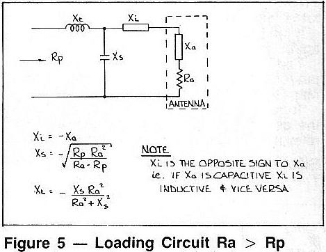
If Ra is greater than the desired load resistance (Rp), use the circuit of Figure 5 and calculate thus:

i. Series reactance Xi = -Xa
That is :-
If Xa is inductive, Xi is made an equal value of capacitive reactance.

If Xa is capacitive, Xi is made an equal value of inductive reactance.


ii. Calculate shunt capacitive reactance (Xs):

Xs = √[Rp.Ra²/(Ra-Rp)]

iii. Calculate series inductance (Xt):

Xt = Xs.Ra²/(Ra² + Xs²)

Fixed capacitance and inductance values are now calculated from the standard formulae:

C= 1/2.π.f.Xc

L= XL/2.π.f


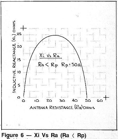
Taking the calculation further, specifically for 1.8MHz, we have worked out curves of network components assuming a transmitter load of 50 ohms. These curves can be used as follows:

If Ra is less than 50 ohms. use the following procedure:

i. Refer to Figure 6 to obtain the value of Xi.

ii. If Xa is capacitive, add its value to Xi to obtain Xt,an inductive reactance.

iii. If Xa is inductive, subtract its value from Xi. If the result (Xt) is positive, Xt is inductive If the result (Xt) is negative, Xt is capacitive.

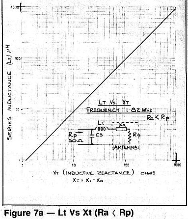
iv. Now find the value of series inductance (Lt) or series capacitance (Ct) from Xt in Figures 7a or 7b respectively.


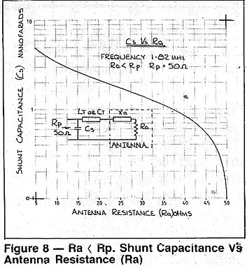
v. Finally, refer to Figure 8 to obtain the value of shunt capacitance (Cs).
If Ra is greater than 50 ohms, use the following procedure:

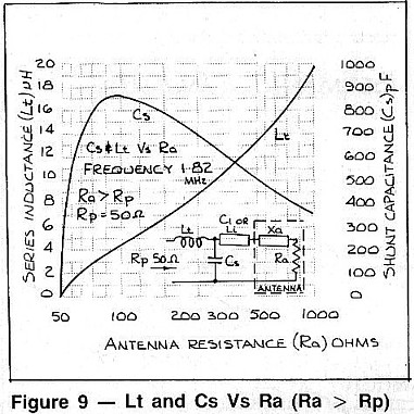
i. Refer to Figure 9 to obtain the value of series inductance (Lt) and shunt capacitance (Cs).

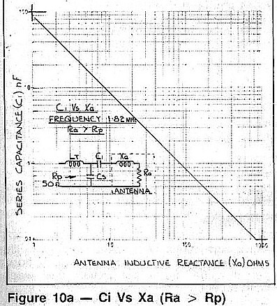
ii. If Xa is inductive, a series capacitor (Ci) is required and its value is selected from Figure 10a.

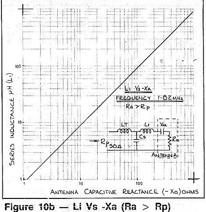
iii. If Xa is capacitive, a series inductance (L1) is required and its value is selected from Figure 10b.

NETWORK COMPONENTS

The network capacitors should have sufficient voltage and current rating. A power of 400W PEP across 50 ohms develops a peak voltage of 200 at a current of 200 V divided by its reactance. A good quality mica capacitor or a large air dielectric tuning capacitor could be suitable.
The series inductor should be made to have a high Q. Its loss resistance causes further power loss and if sufficient in value. compared to the antenna resistance (Ra), its value should be added to all calculations involving Ra. Network calculated values should then be re-assessed. To check the inductance and loss resistance, the noise bridge can again be utilised.

TESTS

If everything has worked out right, the input of the network should look like a resistance equal to Rp (50 ohms) with negligible reactive component. This can be checked by the further use of our valuable noise bridge. If Rp value is correct, our transmitter can be connected and we are ready to transmit.

At this point, with the aid of an RF ammeter and the measured values of Ra and Rp, we can check our matching efficiency. Connect the RF ammeter in series with the transmitter output and, with the transmitter on tune, record the current (It). Reconnect the RF ammeter in series with the antenna and for the same transmitter setting, record antenna current (la).
Transmitter power output is equal to It².Rp and radiated power is equal to Ia².Rr.

Efficiency of the matching network is calculated as:

100.Ia².Ra/It². Rp %

Efficiency of the whole aerial system is calculated as:

100.la².Rr/It².Rp


A possible inaccuracy is the value of Rr, taken from Figure 2 and based on antenna length. Its value for a given length could vary with other physical features of the antenna.

TRANSMISSION LINE

Previous discussion has assumed that the transmitter is connected directly to the antenna tuning network within the radio shack. A disadvantage in doing this is that high RF current flows in the antenna and earth conductors within the shack, causing a high local RF field. Apart from its nuisance value, considerable radiated power could be wasted in absorption in the building structure.

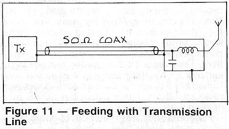
To eliminate this problem, one might choose to place the tuning network external to the shack, directly between the antenna wire and earth or counterpoise and feed via a transmission line, such as a 50 ohm coaxial cable (refer Figure 11).

A point worth noting is that you should not get too concerned at poor standing wave ratio (SWR) on the line at this frequency (1.8MHz). The loss in coaxial cable at 1.8MHz is quite low and even for an SWR of as high as 3:1, the net loss is a fraction of a dB per 100 feet. If the transmitter loading is satisfactory, precise SWR can be ignored.

In conclusion, it can be said that power radiated might not mean power in the direction you would like it to go and that is another subject. However, it is hoped that the information here will be of some help with those loading problems.

LATER FOOTNOTE

If the antenna load resistance (Ra) is lower than the source resistance (Rp), it has been assumed that one must use the circuit of figure 4. However, as a result of later experimentation with the Z Match Tuner, it is now clear that if there is reactance in series with the output load resistance , the load circuit can be considered in the equivalent parallel form with a high parallel resistance component. In this case, the circuit of figure 5 can be applied. This is how the Z Match (which uses the Figure 5 configeration) can match both high and low resistance loads.
,
However there are traps with that arrangement. If the matching system happens to introduce, in the output circuit, a reactance opposite to the inherent series reactance of the antenna load, the reactances cancel and the match is not possible. In the Z Match Tuner, we fixed that problem by providing an extra small inductance which could be switched in to upset the cancellation. (Reference 3).

REFERENCES

(1) "An Approach to Antenna Tuning" by Lloyd Butler VK5BR - Amateur radio, June 1987

(2) "An L of a Network" by Graham Thornton, Amateur Radio, April and May 1995.

(3) (1) The Single Coil Z Match - An Inherent Dropout with Certain Capacitive Loads and how to Fix the Problem, by Lloyd Butler VK5BR and Graham Thornton VK3IY.

APPENDIX
The original article was followed by an appendix which listed the original mathematics I had used with complex algebra (j notation) to derive the formulae for the L Match components. It was really background information not needed for the practical evaluation of the components, so I didn't include it here.

Back to HomePage