|
|
INTRODUCTION
MIXING PRINCIPLE
One only has to examine the output of a mixer on a spectrum analyser to realise that It Is a complex device. Here we examine some of the principles of mixing and mixing devices.
Numerous mixer stages are found in modern transmitters and receivers. These are well-known as devices which produce, from two initial frequencies, additional frequency components equal to the sum and difference of the others. One of these new components is separated from the others by selective tuning or bandpass filters. Actually, a multitude of other frequency components is generated and these must also be considered in the transmitter and receiver design.
All kinds of problems can, occur from the mixing process and if you are interested in experimenting with your own equipment designs, an "in-depth" study of the mixing process is well worthwhile. In the following paragraphs an attempt is made to study some of the basic principles involved.
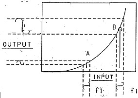
if two signals of different frequency are fed through a linear device, they will appear at the device output as the same two frequencies. To mix two signals we require a curved or non-linear characteristic such as shown in Figure 1. The diagram shows a low-level signal f1 with the operating point set for two positions, A and B. Observe that the output level of fi is much higher when the operating point is set to B than when set to A. Now, examine Figure 2. In this diagram, we sweep the operating point between point A and B with a second high level signal fo modulating the amplitude of fi. The word "modulating" has been deliberately used here to demonstrate that if fi were a carrier frequency and fo an audio frequency, we would call it amplitude modulation. The point being made is that amplitude modulation is the same process as mixing, the sum and difference components being the sideband components referred to in modulation.
|
|
MULTIPLICATION
MIXING PRODUCTS
Referring again to the discussion Figure 2, the process of mixing is mathematically one of
multiplication. The instantaneous amplitude of fi is multiplied by the instantaneous amplitude of
fo, hence the resultant components are called products. This is all very confusing as we know
that the frequencies formed are equal to sums and differences. It must be understood that it is
the Instantaneous amplitudes which are multiplied, not the frequencies and the phenomenon can be explained by using one of the well-known trigonornetric identities:
sin(A) sin (B) = (1/2) cos(A + B) - (1/2) cos(A - B) ... (1)
We can express, the instantaneous amplitude of f1 and fo as follows:
Ai.sin(2π.fi.t) and Ao.sin(2π.fo.t)
where Ai and Ao are their respective amplitudes and t = time.
Multiplying them together by substitution in the identity (1), we get the following:
Ai.sin(2π.fi.t).Ao.sin(2π.fo.t)
= (1/2)AiAo{cos[2π.t(fo + fi)]- cos[2π.t(fo - fi)]}
We can see that two new cosine functions of (fo + fi) and (fo - fi) are formed which represent our sum and difference frequencies. Of course, a cosine wave is the same as a sine wave, with the time scale simply shifted by 90 degrees.
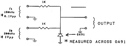
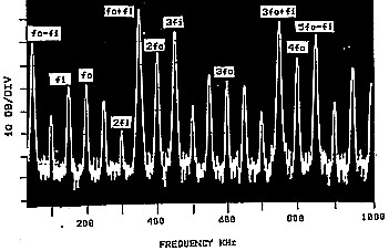
At the output of a mixer, there are many more components than the sum and difference of the input frequencies. To illustrate these on a spectrum analyser, a simple mixing circuit, using a germanium diode, was set up as shown in Figure 3. Signal fo was set at 1 VPP across the diode, just sufficient to sweep the operating point of the diode over the curvature of its voltage versus current characteristic and signal fi was set lower at 0.1 VPP The two frequencies of I50 kHz and 200 kHz, used for fi and fo respectively, are of no particular significance other than to demonstrate the effects.
 |
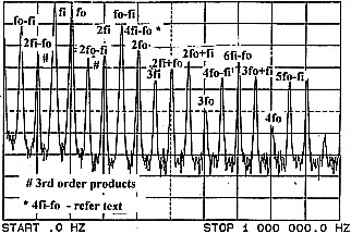
 (Voltages across diode - fo = 1Vpp, fi = 0.1vpp) Y Scale on graph - 10 dB per division. |
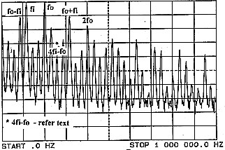
 (Vo1tages across diode fO = 1 VPP, fl = 1 VPP) Y scale on graph is 10 dB per division. |
 (Voltages across diode: fo = 1Vpp, fi = 1Vpp) fi is changed to 115 kHz Y scale on graph is 10 dB per division. |
 CM1 Full Ring |
 |
MIXING MODES
Mixers can be classified as those which operate in a continuous non-linear mode, as shown in Figure 2, or as those which operate in the switching mode.
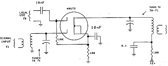
A typical continuous non-linear mode mixer is the dual gate MosFET circuit as illustrated in Figure 9. The MosFET has a square law characteristic which is particularly good for mixing purposes. Because of its high gate impedance, it requires little power to drive it and the separate gates provide good isolation between the two signals being mixed.
 |
SWITCHING MODE MIXERS
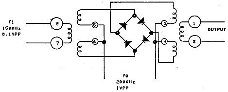
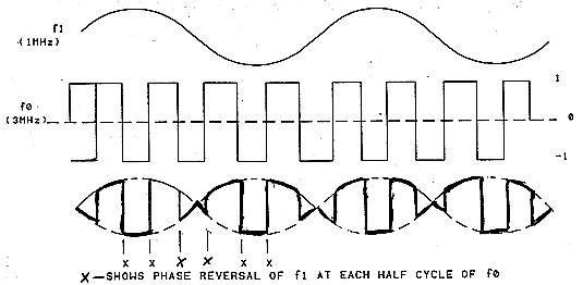
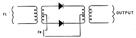
The second classification of mixer to be discussed refers to those which operate in the switching mode. These mixers operate by switching one input signal (f1) between two states at each half cycle of the second signal (fo). Figure 7 illustrates a double balanced switching mode mixer in which diodes act as switches. Pairs of diodes are biased on alternately each time the polarity of fo reverses and this reverses the phase of f1. The switching process is illustrated in Figures 10 and 11, the first showing fi a higher frequency than fo and the second showing fi lower than fo The signal fi is actually multiplied by a square wave of frequency fo, an amplitude equal to one and comprising a fundamental and harmonic component as follows:
(4/π)[cos(2π.fo.t) - (1/3)cos(2π.3fo.t) + (1/5)cos(2π.5fo.t) ... etc] ----------------(2)
that is, fi is multiplied by the fundamental of fo and all its odd harmonics. (Note that a perfect square wave has no even harmonics).
It is significant that the square wave has only two states, one and minus one, so that to multiply with fi it is only necessary to multiply fi alternately by one and minus one, that is, reverse the phase of fi at each fo polarity transition.
This mixer is defined as double balanced because both input signals are balanced out from the output. The reduction of the level of these in the output was previously referred to and illustrated in Figure 8.
 Double Balanced Mixer Commutation of f1 by fo ( fi higher than fo) |
 Double Balanced Diode Mixer Commutation of fi by fo (fi lower than fo). |
 |
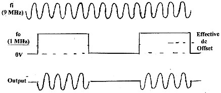 (fi is multiplied by switching wave fo and a DC offset equal in amplitude to the switching wave) |
OUTPUT
The degree of input signal isolation in the balanced mixer is determined by the accuracy of transformer balance and the degree of matching of the diodes. Before the solid state era, some carrier telephone systems used copper oxide metal rectifiers. Modern balanced mixer modules, suitable for VHF and UHF, use hot carrier diodes which are characterised by low conduction voltage, low reverse current, low capacitance and very high frequency performance.
Diodes of all types have a curved turn-on characteristic and unless driven hard by signal fo will operate in a partial continuous non-linear mode. In the balanced mixer spectrum, shown in Figure 8, even harmonics of fo are evident indicating that perfect square wave switching is not taking place.
Diode balanced mixers work very well but have conversion loss rather than gain. They are also low impedance devices and require low source impedance circuits to drive them. Because of these characteristics, active balanced mixers, using bipolar or field effect transistors, are often used. These have conversion gain and can be driven by higher source impedance circuits.
An active balanced mixer, built by the author for use in a transceiver, is shown in Figure 14. In this application, a 4 MHz SSB signal was upmixed to 17 MHz by beating with a 21 MHz carrier. The spectrum for this mixer is illustrated in Figure 15. This mixer works in continuous non-linear mode with signal fo swinging the gate voltage over a large section of the drain current versus gate voltage characteristic. Fine balance of transistor gain is achieved by differential adjustment of drain current with the bias adjustment potentiometer in the source circuit.
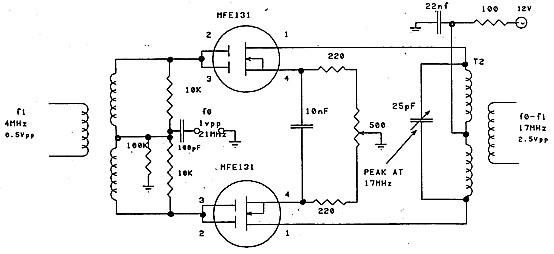 T1 -10 turns tri-filar wound on philips toroid 97120, μ = 2300 T2 - 8 turns tri-filar wound on philips toroid 97160, μ = 120 |
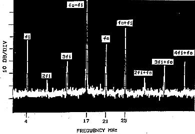 Spectrum Analysis of MosFET Balanced Mixer |
UP MIXING AND DOWN MIXING
INTERMODULATION PRODUCTS
THIRD ORDER INTERCEPT
The question can be asked, when, does one use a balanced mixer in preference to a non balanced type? One answer lies in how difficult it is to remove the reference carrier with tuning or filtering. In the case of Figure 14, the 21 MHz carrier is very close in frequency to the 17 MHz product required and the balanced circuit was built in after some difficulty was experienced with the high residual carrier level at the output.
The same frequency conversion, in reverse, was required in the receiver where conversion was from 17 MHz down to 4 MHz using the same 21 MHz carrier. In this case the 21 MHz is well removed in frequency from 4 MHz and no problem was experienced in using an ordinary dual gate MOSFET mixer similar to Figure 9.
The point being emphasised is that a balanced mixer is more likely to be required when up rnixing, as required in an SSB transmitter, than when down mixing in the matching receiver. Another use of the balanced mixer is that of an amplitude modulator which generates double sideband suppressed carrier signals. Signal f1 is then the speech input and the carrier fo is balanced out. In this application the mixer is normally called a balanced modulator. Remember that we have already said that mixing and amplitude modulation is the same process. The balanced modulator is the first stage in our single sideband transmitter to generate two sidebands, one of which is removed by a selective filter.
Because our mixing device operates in a non-linear mode to carry out its function as a mixer, it can also generate intermodulation products from unwanted signals at its input. The products might result from mixing our signal fi (which we will now call f1) with some other signal f2 or from mixing together two entirely different signals f2 and f3. The most troublesome of these are what are called the third order products (2f1-f2) or (2f2 - f1). These are troublesome because they are normally the closest intermodulation products to our desired signal f1.
Suppose our desired signal f1 is 14.200 MHz and another signal f2 is present on 14.300 MHz. In this case, our third order products are at 14.100 MHz and 14.400 MHz. Suppose there were a third signal C on 14.400 MHz and we calculate the third order products from f2 and f3, that is, (2f2 - f3) and (2f3 - f2). From these we get 14.200 MHz and 14.500 MHz the first of which is the same frequency as our desired signal f1 and a cause of interference.
Clearly interference from intermodulation products can be, a serious problem and one measure of performance of a mixer is the level of its third order products at the output relative to the desired sum or difference product.
it was suggested in earlier paragraphs that to keep intermodulation products low, It was necessary to operate the input signal fi at low level. We will now examine the reason for this.
Suppose we feed two sine wave signals of equal amplitude to the input of a non-linear device. We take note of the level and then increase the level by a factor of 3.16 (or 10 dB). Because of the non-linearity, the change in output level will not be the same as the change in input level, however the output can be resolved into components consisting of the two fundamental frequencies f1 and f2, and other components which can all be examined separately The fundamental frequencies must increase linearly otherwise they would not be fundamentals and hence their outputs increase by the same factor as the input (i.e. 3.16). The other components will follow some other law.
In previous paragraphs we referred to the trigonometry identity cos(2A) - 1/2(sin**2A) and showed that second harmonic components are associated with a sine squared function, hence we can conclude that second harmonic components 2f1 and 2f2 follow a square law function of the input level. Of course at this stage, we are really interested in the third-order products, the results of multiplying 2f2 by f1 and 2f1 by f2. With fi and f2 equal in amplitude, the result is that our third order products (2f2 - f1) and (2f1 - f2) follow a cube law relationship with the input level. Tabling our input change of 3.16 in decibels, we get the following:
Change in input level - 20 LOG 3.16 - 10 dB
Change in output at fundamental - 20 log 3.16 = 10 dB
Change in output of third order products = 20 log 3.16**3 = 30 dB
Because the third order intermodulation products increase with the cube of the input change, as compared to the linear change for the fundamentals, the higher the signal level input, then the higher the ratio of intermodulation products to fundamental. There is also a theoretical point where the output level of intermodulation products equals the output level of the fundamental. This point is called the Third Order Intercept Point and this is often specified to define the third order lintermodulation performance of a mixer.
To measure the intercept point, we set up the equipment as shown in Figure 16. Two calibrated signal generators of equal signal level are fed to the inputs of the mixer and the output monitored with a calibrated spectrum analyser. As the device is a mixer, both fundamental and third order products are shifted in frequency by a value fo (the local oscillator frequency). In the case of Figure 16, the relevant output components are the Desired Signal (fo - f1) and the Third Order Components [fo - (2f1 - f2)] & [fo - (2f2 - f1)]
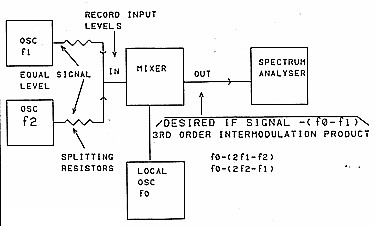 Test Set Up to measure Mixer Performance |
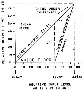 Showing Third Order Inter-Modulation Intercept. DR = Dynamic Range for no discernable IMD products |
NOISE LEVEL AND DYNAMIC RANGE
Using the test equipment, Figure 16, another important measurement is the level of the noise floor at the output. As previously discussed, the lower the input signal level, the lower the level of intermodulation products. However, the lower the signal level, the lower the signal to noise ratio.
In Figure 17, the noise floor is recorded as 0 dB output and this information, together with levels of signal and intermodulation products, is transferred to a different form in Figure 18. Here we show the signal to noise ratio as a function of input signal level on one curve and the ratio of signal to intermodulation products as a function of input signal level on the other. Observe that there is an optimum operating level where the curves cross and where the output signal is 50 dB above both the noise and the IMD products.
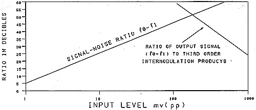 Comparison of signal to noise ratio and signal to Intermodulation product |
SUMMARY
Mixers can be categorised in the following ways:
1. Operation in a continuous non-linear mode or operation in the switching mode.
2. Unbalanced operation or balanced operation in which one or both input signals are balanced out at the output.
3. Mixers which have conversion gain and mixers which have conversion loss.
Mixers are usually best operated by sweeping the reference signal fo over the full non-linear region of the mixer characteristic curve but operating the input signal (f1) at a lower level, sufficient to give good signal to noise ratio but low enough to minimise intermodulation products.
Third order mixer products rise in proportion to the cube of the input signal level (and output signal level). Mixer performance as a function of signal input level can be defined by the third order intercept point and the noise floor level.
What we have presented here is an exploration of how mixers work and a few ideas on how they should be operated. Further information on the practical application of these devices can be found in handbooks such as published by the American Radio Relay League (ARRL).