Extreme narrow bandwidth techniques

Extreme narrow bandwidth techniques ON7YD

About this page :
The main object of this page is to provide information. It has been deliberately kept simple, no fancy and flashy tricks, in order to achieve maximum compatibility for the different browsers and to allow fast downloading.
Any comments and/or suggestions are welcome at : [email protected]

Translated versions

Russian (by UA3VVM)	:	http://www.cqham.ru/qrss.htm
German (by DL2WRJ)	:	http://www.dl2wrj.net/technik/narrow/136narrow.html
Italian (by IZ8BZX)	:	http://www.iz8bzx.info/136narro.htm
Japanese (by JH1GVY)	:	http://www003.upp.so-net.ne.jp/JH1GVY/Enbt.htm
French (by F8ARR)	:	in preparation

last updated on 30 August 2005

Index

Introduction
Bandwidth
Digital Signal Processing (DSP)
1. DSP basics
2. Fast Fourier Transform (FFT)
Extreme narrowband modes
Jason : a "keyboard to keyboard" mode
WOLF : an alternative route
Nihil novum sub sole
Available software
Operating practice
Literature
Acknowledgements

1. Introduction

Due to several reasons the signal to noise ratio (SNR) of ham signals on 136kHz is often very low :

A wavelength of about 2.2km (1.35 mile) makes any ham antenna small and inefficient.
1 Watt ERP power limit
High noiselevels
Strong commercial stations (100kW and more) very close to the ham band

One way to improve the SNR is to reduce the receiver bandwidth and thus have less unwanted signals and noise while leaving the level of the wanted signal unchanged. But the reception of any signal requires a minimal receiver bandwidth depending on the type of modulation. SSB has a typical bandwidth of 2.4kHz, the bandwidth of a CW signal is dependent on the speed but in any (practical) case less than 100Hz. The use of a filter with a narrower bandwidth than that of the transmitted signal will distort the signal.
Here I will describe a technique that allows to communicate with signals far below the noise level. It can be used to make a basic QSO and I think that in some way the 'value' of such QSO's can be compared to Meteor Scatter QSO's on VHF.

2. Bandwidth

The dominant and most efficient mode on 136kHz is CW. As mentioned before the minimal bandwidth at the receiver side is determined by spectrum of the transmitted signal. In case of CW it is the (keying) speed that puts a limit to the minimal bandwidth.
An accepted method to measure the speed of CW is the PARIS system. The word Paris has a length of exactlty 50 'dots', word spacing included. Based on this system a CW signal of 12 words per minute (WPM) means 600 'dotlengths' per minute or 10 'dotlengths' per second. But as each dot is separated by space of the same length the actual length of the 'dot-cycle' is the double. If a continious series of dots is given at 12WPM this results in a 5Hz square wave. If an RF signal is keyed with this series of dots you will get a carrier with 2 sidebands at 5Hz, resulting in a 10Hz wide signal. Depending on how 'hard' the keying is more sideband further away from the carrier will be created but these do not contain additional information and can be considered as a waste of energy (and a source of QRM to others). So basicaly the minimum bandwidth that is required to receive a CW signal undistorted is :

B = 0.833 * WPM (Hz)

Assuming that the only noise source is a frequency independent (white) noise, the total receiver noise will be directly proportional to the receiver bandwidth. Taking a 12WPM CW signal as a reference and assuming that the receiver bandwidth is optimized to the transmission speed the table below shows the SNR improvement that can be achieved by reducing the CW speed :

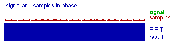
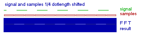
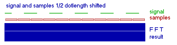
Speed	optimum bandwidth	SNR vs. 12WPM
12WPM	10Hz	0dB
8WPM	6.67Hz	+1.8dB
4WPM	3.33Hz	+4.8dB
1 sec./dot	1Hz	+10dB
3 sec./dot	0.33Hz	+14.8dB
10 sec./dot	0.1Hz	+20dB

It is clear that a significant SNR improvement can be achieved by reducing the CW speed. On 136kHz a dotlength of 3 seconds has become a kind of standard and this mode is called QRSS (from the Q-code QRS : please reduce your speed). At these very slow CW speeds it becomes rather difficult to copy the signal by ear as you would almost need a chronometer to time the dots and dashes. Furthermore the frequency of the signal needs to be very stable as smaller bandwidths are used. Fortunately this not a big problem on 136kHz where a frequency stability of 0.1Hz is rather easy to achieve.
Another problem is that filters become more and more complicated to built as the bandwidth becomes smaller. And also tuning into a signal can be a rather tricky thing at bandwidths below 1Hz.
So reducing bandwidth not only has benefits in the way of an improved SNR but creates also a lot of additional problems. One way to overcome many of these problems is the use of Digital Signal Processing (DSP).

3. Digital Signal Processing (DSP)

3.1. DSP basics
Digital Signal Processing is one of these magic expressions that you hear once in a while, but seems the domain of specialized electronic engineers and maybe some 'happy few' hams. Until very recentely special (and rather expensive) hardware was needed to perform DSP. But now all the special hardware can be replaced by a pentium PC with soundcard and the software you need is available for free. Practical details can be found here. As the expression Digital Signal Processing says, the analog (input) signal is converted to digital, then processed and eventually converted back to an analog (output) signal.

The conversion of the analog signal to a digital form is done by analog-to-digital conversion (ADC). The most basic version of ADC is often done by ourselves when we use a voltmeter to determine the value of a voltage. With DSP this 'reading of voltages' is done automatically at a known time interval, this is called sampling. The result is a series of measurements, where we know the measured voltage and the time when it was measured.

These data are processed digitally, what in practice means that they undergo a series of more or less complicated calcualtions. The result can be interpreted as digital data or eventually converted back to an analog signal. Using DSP all kind of things can be done, not only filtering but also reducing bandwidth, time multiplexing of several signals etc...
Here we will only discuss the filtering of a signal.

3.2. Fast Fourier Transform (FFT)
Althought there are several methods to filter a signal digitally the major technique is by using Fast Fourier Transform (FFT). The mathematical background on this transform was developed by Joseph Fourier, about 200 years ago. The basic idea behind this transform is that any signal can be seen as the sum of a series of sinusoidal signals, where each sine can have a different amplitude and phase.

In the above picture the complex red signal is equal to the sum of the green, blue, orange and black sines. The mathematical equations of the Fourier transform are rather complicated, those who are interested can have a look at following webpages :

Frequency Domain Analysis - Basic Concepts and Definitions (King Fahd University of Petroleum & Minerals) : complete, but it takes some math
FFT for dummies (by Renato Romero, IK1QFK) : mainly visual explanation of FFT, very good for beginners

Fortunately it is not necessary to go deep into these mathematics to understand how FFT works and therefore the maths will be kept to a minimum. But as there is a lot of calculating involved Fourier transforms will take a lot of 'computing time'. To reduce this a special algoritm was developed to enhance the speed of the Fourier transforms, this algoritm is called the Fast Fourier Transform (FFT).
When we take the Fourier transform of any signal we actually split the signal up in a number of sines and for each of these sines the amplitude and phase is calculated. Each of these sines represents a certain frequency (or better frequency band) and from these sum of sines (and their amplitudes) we can reconstruct the frequency spectrum of the measured signal.

The 'quality' of the reconstructed frequency spectrum depends on 3 things :

the sample rate (interval between 2 A-D conversions)
the sampling time for one transform
the number of bits of the A-D convertor

The sample rate determines the maximum frequency of the spectrum : the maximum frequency that can be reconstructed is 50% of the sampling frequency.
eg. : If we take a sample every 0.2ms (equals a sampling frequency of 5kHz) the maximum frequency that can be reconstructed is 2.5kHz.
The sampling time determines the frequency resolution (or the bandwidth of each 'channel') : the frequency resolution is equal to one over the sampling time.
eg. : If we take a sampling time of 0.1 seconds the frequency resolution (or channel bandwidth) will be 10Hz, this means that in the series of sines of the Fourier transform each sine will represent a 10Hz wide channel.
The number of samples in a Fourier transform has to be a power of 2 (2, 4, 8, 16, ... , 256, ... 65536, ...). Although you can take any number of samples and just add a series of 'zeros' until you get a power of 2 it is more practical to choose the correct ratio between sample rate and sampling time in order to get the right number of samples.
eg. : if we have a sample rate of 0.2ms we will not take a sampling time of 0.1 seconds, what would result in 500 samples, but a sample time of 0.1024 seconds in order to get 512 samples (= 2⁹). The result of the Fourier transform will be a series of 256 sines where each sine represents a 9.766Hz wide channel between 0Hz and 2.5kHz.
The picture below shows a simple example, the Fourier transform of 16 samples at a rate of 1ms results in a series of 8 sines that each represent a 62.5Hz wide channel between 0 and 500Hz :

The number of bits of the A-D convertor determines the dynamic range of the spectrum. In practice (using the PC soundcard) we can choose between a 8-bit or 16-bit A-D conversion.
eg. : For a 8-bit A-D conversion we have 2⁸ = 256 levels and the dynamic range will be 20.Log(256) = 48dB. For a 16-bit A-D conversion we have 2¹⁶ = 65536 levels and the dynamic range will be 20.Log(65536) = 96dB.

4. Extreme narrowband modes

4.1. QRSS

4.1.1. What is it ?
QRSS is extreme slow speed CW, the name is derived from the Q-code QRS (reduce your speed). To take advantage of the very narrow bandwidth of the transmitted signal an appropriate filter at the receiver end is needed. Making a 'software filter' using FFT has some advantages over the oldfashioned hardware filter. One of the main advantages, when using it for reception of slow CW signals, is that FFT does not give you one single filter but you get a series of filters with which you can monitor a complete spectrum at once. This means that you do not have to tune exactly into the signal, what can be very delicate at sub-Herz bandwidths. Also it is possible to monitor more than one QRSS signal at the same time. At first glance it looks as if it is complicated to do this, even if FFT presents you this nice multi-channel filter it might be difficult to monitor all these channels. Further the long duration of the dots and dashes is unfavourable for aural monitoring.
A solution to the above problems is to show the outcome of the FFT on screen rather than making it audible. The result is a graphic where one axis represents time, the other axis represents frequency and the color represents the signal strength. If the vertical axis represents time we call it a waterfall display while it is called a curtain display if the horizontal axis represents time.
All this may sound complicated but it is easy to understand when you see an example (curtain display) :

The picture above shows the signal of HB9ASB who was not audible due to very strong QRN, the vertical lines are the result of S9++ static crashes.
Some nice collections of screen captures can be found at the webpages of DK8KW, G3XDV, OK1FIG and NL9222

4.1.2. Comparing dotlength and SNR (practical results)

4.1.2.1. By DK8KW
In April 2000 Geri Kinzel (DK8KW) did some measurements to compare QRSS with normal (aural) CW :
This morning I made some laboratory tests to get some indication about the ability to communicate with signals below noise level using QRSS. I used a calibrated frequency synthesizer (Adret 2230), an 0-120 dB attenuator in 1 dB steps (Schlumberger BMD500) and my Praecitronic MV61 Selective Level Meter. With a BNC T-connector I fed the normal band noise including LORAN lines on 137.500 kHz (+/- 50 Hz) to one side and the output of the frequency synthesizer to the other side. With the attenuator I made sure that a 0 dBm (50 Ohm) signal with the synthesizer corresponds to a -80dBu ( 0dBu = 0.775V into 75 Ohm = +9dBm, -80dBu = -71dBm) signal at the MV62 (plus/minus 1 dB). The band was quite, with a background noise around -110dBu (S4, -101dBm) and LORAN lines clearly visible. Using the 100 Hz bandwidth of the MV62 and the cascaded 250 Hz/500 Hz CW filters of the IC-746 I checked the signal by ear as well as with the Spectrogram software with the normal parameters I use for "3-5 second-dot-length" QRSS (5.5k sample rate, 16bit mono, 16384 points FFT = 0.3 Hz resolution, 60 dB scale, 300 ms time scale, 10 x average) and obtained the following results:

Signal strength at RX input	Comment
-100dBu / -91dBm	good audible CW (S6)
-110dBu / -101dBm	CW signal equal to noiselevel (S4), can just be copied
-115dBu / -106dBm	boundary for aural CW, signal just detectable by ear
-125dBu / -116dBm	perfect readable QRSS signal ('O' report)
-130dBu / -121dBm	good readable QRSS signal ('M' report)
-135dBu / -126dBm	just detectable QRSS signal ('T' report)
-140dBu / -131dBm	signal not detectable

Conclusions:
QRSS has a 20 dB signal level advantage over normal (aural CW), which means that the minimum detectable and/or readable QRSS signal that might just allow communication lies 20 dB below the signal, that can just be detected and/or decoded by a trained CW-operator's ear. If I consider the "CW-operator's ear/brain bandwidth" to be 30 Hz, this roughly corresponds to the bandwidths used (0.3 vs 30 Hz).

4.1.2.2. By W1TAG
John Andrews (W1TAG) did also some measurements. He was using an Icom R75 receiver and 6 foot loop to receive the signal transmitted by a 10 mw exciter, feeding a small loop antenna through a variable attenuator. The receiver was picking up whatever noise was present at the time of the test. The signal was decoded using the ARGO software.
The transmitted signal was attenuated to a level that just allowed a solid copy :

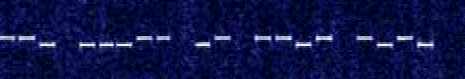
Dotlength	Measured level (vs. 6WPM)	Theoretical level (vs. 6WPM)
0.2 sec. (6 WPM)	reference	reference
3 sec.	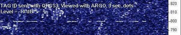-10dB	-11.8dB
10 sec.	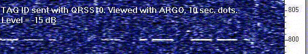-15dB	-17dB
30 sec.	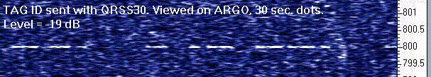-19dB	-21.8dB
60 sec.	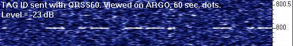-23dB	-24.8dB

For all measurements there is a +/- 2dB difference between the measured and theoretical result, but I believe that this can be explained by the fact that the 6WPM reference screenshot has a clearly lower SNR than the other screenshots. The full report on this measurement can be found here

4.1.2.3. By G3YXM and G3NYK
In March 2002 G3YXM and G3NYK compared normal CW and QRSS at speeds of 3 sec/dot, 10 sec/dot and 60 sec/dot over a 220km path. G3YXM was transmitting and reduced power until it just reached the "O copy" level at G3NYK :

Dotlength	Power into antenna	Improvement vs 12WPM CW	Theoretical value
0.1 sec. (12WPM)	360mW	reference	reference
3 sec.	23mW	12dB	14.8dB
10 sec.	3.9mW	19.7dB	20dB
60 sec.	0.6mW	27.8dB	27.8dB

The full report of this test can be found here.
Dave states that he needs to run 2kW RF into his antenna to achieve 1W ERP. This means that the ERP at the 60 sec/dot test was no more than 300nW (yes, nano-Watt), not bad at all to cover a distance of 220km.

4.2. Dual Frequency CW (DFCW)
At a speed of 3 seconds per dot a very basic QSO will take about 30 minutes. Changing QRN levels and/or propagation during this period can have a vast effect on a QSO. Therefore a new transmission mode has been developed that enhances the average speed by a factor of 2.5 to 3.
When the nature of CW is analyzed it seems a digital mode where 'key down' respresents a logic '1' and 'key up' a logic '0'. But another approach it is to see it as a mode with 3 'logical states' : the 'dash' (3 periods of key down + 1 period of key up or '1110'), the 'dot' (1 period of key down + 1 period of key up or '10') and the 'character space' (2 periods of key up or '00'). The spacing between words is 3 character spaces. So there are 2 elements that play a role : the presence/absense of a signal and the duration of the signal. As CW was intended to be received by ear the different duration of the signals is essential, but it lengthens the time needed to transmit a text.
In Dual Frequency CW (DFCW) the element 'duration' is replaced by the element 'frequency'. So dots and dashes no longer have a different length but they are transmitted on a different frequency. Due to this frequency shift there is no 'space' needed between the dots / dashes and the character space can be reduced to the same (dot)length.
When the idea of DFCW first was introduced there was a lot of scepticism about the readablility of there frequency shifted signals but in practice it seems rather easy to read it from the screen. To make it even more easy to read, especially during a sequence of dots ot dashes, a short space (typicaly 1/3 of a dotlength) is added between the dots and dashes. This reduces the average speed a bit, but is improves the readability and also reduces the duty cycle (what is better for the PA).
The example below show the text 'CQ ON7YD K' in QRSS and DFCW, at the same speed :

At a speed of 3 seconds per dot this CQ will take 5'30" in QRSS while it will take only 1'54" in DFCW. The speed advantage of DFCW over QRSS can be taken in 2 ways, either by reducing the duration of a QSO or by increasing the dot length and working at a narrower bandwidth. The last means that, for the same duration of a QSO, the dot length in DFCW can be 2.5 to 3 times longer and as a result of this get a 4 to 5dB better SNR.

The screenshot below shows a 'real-world' picture of a DFCW signal. I hope this proves how easy it is to decode a DFCW signal by eye.

4.3. Future developments of extreme narrowband modes
Over the past year a dot length of 3 seconds has become a kind of informal standard for QRSS and DFCW, as practical test have shown best results for this speed. Most hams use the Spectogram software at the receiving end with a sample rate of 11kHz and blocks of 16384 samples, this means a sample time of about 1.5 seconds. At first sight it is not so obvious why the sample time is only half the dot length, wouldn't it be better either to make the sample time longer or the dot length shorter ?
But there is a good reason why the sample time is so much shorter than the dot length, it is because so far the transmitter and receiver do not work 'synchronised'. This means that a sample block (at the RX end) begins somewhere in the middle of a dot (at the TX end) and vice versa. What happens when dot length and sample block have the same duration is shown in the pictures below :

To ensure that at least 1 sample block falls completely within each dot (or dash, space) a sample block can not be longer than half the dot length.
If we can create some kind of 'synchronisation' between TX and RX it would be possible to (almost) double the sample block duration without increasing the dot length and thus achieve a 3dB gain. When DFCW is used and the dot length is increased to 10 seconds a QSO will take about the same time as a 3 sec./dot QRSS QSO. Assuming that it should be not so difficult to 'synchronise' transmitter and receiver software with a 1 second accuracy a sample block of 8 seconds (with a 2 seconds interleave) and a dot length of 10 seconds seems possible to me :

Compared to the 'traditional' QRSS a gain of over 7dB can be achieved while the duration of the QSO is about the same. Timing errors (between TX and RX) upto 1 second will not affect the SNR.

An alternative solution is given by the programmers of Spectran. Instead of using a complete new set of samples for each FFT they take only partly new data and 'shift' the existing data up in the data-array used to perform the FFT:

eg. : Assume that 4096 datapoints are used to perform a FFT. Instead of using a complete new set of data for the next FFT you remove the 128 'oldest' points (that are in position 3969 to 4096 in the data-array), shift the datapoints in position 1 to 3968 upward to the end of the data-array and fill positions 1 to 128 with new data. This procedure is repeated for every FFT.
This method has the advantage that the 'duration' of the FFT array can be almost as long as the duration of a dot, but there are also some disadvantages. First of all the workload for the computer increases significantly, in case of the above example the computer has to perform 32 FFT's in the time that with the 'traditional' method only 1 FFT calculation is needed. On screen this method also causes some 'blur' at the beginning and end of the dots :

Another way to improve the SNR is averaging. It is based on the fact that noise is random and cancels itself out over a number of measurements while the signal is consistent. Therefore the results of several FFT's are added and the average is taken. While the advantage is an improved SNR the disadvantage is that the results on screen appear slower, as you have only 1 output to screen for several FFT's. Fortunately there is a way arround this, but it has also some drawbacks. Alberto di Bene (I2PHD), one of the programmers of Spectran, sent me some interesting comments on how averaging can be done :
In Spectran there are two averaging mechanisms :

A) the averaging that you can activate with the AVG button on the main panel. This has two sub-choices : the sliding window and the integration radiobuttons. With the sliding window a moving average is performed on the computed spectrum, and a result is output for each input spectrum, no matter what the averaging factor is. This factor has only the effect of adjusting the width of the moving window. On the contrary, when doing integration, if the the averaging factor is N, an output spectrum is generated every N input spectra, simply taking their average.
B) the averaging which is produced as a side effect of the overlapping done on the input time series. The purpose of this overlapping is to produce an output in a time shorter of what would otherwise be needed, should overlapping not be used. To clarify a little : suppose that the sampling rate is 8000 Hz, and the resolution set to 0.12207 (rounded in the display to 0.12) Hz. This implies that the Nyquist frequency is 4000 Hz, and you have 4000 / 0.12207 magnitude values, obtained with 8000 / 0.12207 complex values (the real and the imaginary parts). So you have to compute 8000 / 0.12207 = 65536 complex values, corresponding to an equal amount of real time samples. The time needed for this is 65536 / 8000 (the number of samples you get each second) = 8.192 seconds. And, actually, if you set Spectran with the speed slider at its minum (the slider colour changes to green), i.e. an overlapping factor of 1, you will have a refresh of the screen about every 8 seconds. Things go worse with increasing resolutions, the wait time increases proportionally. If a faster refresh rate is desired, the overlapping can be of help. With this method, you don't wait that a complete new set of input values is ready, but a part of the old data is reused, together with some new ones. Of course there is a compromise (no free lunch...) : in reusing the old data, you loose some time resolution, and this appears on the screen as a smearing, or blurring, of the spectral lines. This effect increases with the overlapping factor. With factors up to about 8, it is not very noticeable, but things go worse with higher values. It's the price to be paid for having a quicker refresh rate. As with almost any choice in life, a suitable compromise must be found, and this has also implications on the optimal dot/dash length.

5. Jason : a "keyboard to keyboard" mode

5.1. About Jason
Jason is developed by the authors of ARGO, one of the most popar QRSS viewers (I2PHD and IK2CZL). It uses the extreme narrow bandwidth techniques as used in QRSS and DFCW in a "keyboard to keyboard" mode, what means that at the TX side you type a text and the it RX side this text appears on the screen.
The basic idea behind Jason is that a character set can be defined by a series of "tones". This kind of coding is rather old, already in 1957 a mode called Piccolo was based on this principle, later followed by modes such as PGP-1 and PUA-43.
In the modes mentioned above each "tone" is characterised by an absolute frequency. At relative high data-rates and sufficient frequency spacing between the tones the required frequency stability and accuracy is acceptable. But when one want to dig deep into the noise the data-rate must be very slow (as learned from QRSS) and on 136kHz bandwidth is limited. Both limitations make the use of an Absolute Frequency Keying (AFK) mode difficult.
The alternative used by Jason is Incremental Frequency Keying (IFK) : not the absolute frequency of a tone but the frequency difference (shift) between 2 subsequent tones is used. This allows much more flexibilty for both frequency accuracy as frequency stability.
16 different frequency shift are used, ranged from 0.252Hz to 4.037Hz in 0.25234Hz steps. The frequency shift is in principle positive (toward higher frequency), but this would mean that the signal would be "running away"" from the initial frequency. As this has to be avoided a simple trick is used : if the frequency moves more than 4.037Hz (= 16 steps) away from the initial frequency it "rolls over" back to the initial frequency. This may sound complicated, but an example will make things clear :

The default center frequency of Jason is 800Hz, with a total range from (800 - 8 steps) = 797.981Hz to (800 + 8 steps) = 802.019Hz. The default center frequency is slot Nr. 8, and the slots are numbered from 0 to 16, for a total of 17 slots.
Assume we start at 800Hz (= center frequency) and the first shift is 6 steps (= 1.514Hz), now the frequency is 801.514Hz, corresponding to slot 8 + 6 = 14.
The second shift is 5 steps (= 1.262Hz), resulting in a frequency of 802.776Hz. Note that the slot number would be now 14 + 5 = 19, which is greater than the maximum slot number 16. So the 5 steps are split up in 2 steps upward (to slot 16), the 3rd step is the "roll over" to slot 0 and finaly the 4rd / 5th step are again 2 step upward to slot 2. The result is a negative shift of 12 steps (3.028Hz) but Jason knows that this has to be interpreted as a positive shift of 5 steps.
More mathematical : if the upper limit is exceeded the correct slot number is computed modulus 17. In this case, instead of shifting to the non-existing slot 19 the shift goes to slot 19 - 17 = 2, corresponding to a frequency of 797.981 + 2 * 0.25234 = 798.468Hz.

As a result the total bandwidth used by Jason is 4.28Hz. More details on the coding used are given in the next chapter (Inside Jason).
The advantage of using IFK is that the requirements on frequency stability and accuracy are rather relaxed, at least at 136kHz. The frequency drift over a 10 minute period should be less than 4Hz what equals about 30ppm at 136kHz. In addition Jason has a kind of Automatic Frequency Control (AFC) built in, giving a lock-range of 12Hz.
Further Jason has also frequency adjustment tool built, what is very convenient for manual frequency tuning.

5.2. Inside Jason
Jason expects an audio signal around a certain frequency. The default frequency is around 800Hz, but this can be changed within the range of 50 to 5000Hz. This signal fed to the soundcard input (ADC, analog-to-digital conversion) and is sampled at 11025Hz. From there on all signal processing is done by software.
Before the actual signal analysing is done the input signal undergoes a series of operations :

First the signal is down-converted (mixed) to a much lower frequency, 10.77Hz. This is done using a NCO or Numerically Controlled Oscillator (simplified : a software oscillator based on a lookup table) that feeds a mixer. The NCO provides 2 signals that are 90� phase-shifted and both feed a mixer that down-converts the signal provided by the ADC.
Next the both signals are sent through a low-pass filter (FIR or Finite Impulse Response filter) that cuts off all frequencies above 17.22Hz.
Finally the sample rate is reduced from 11025Hz to 43.07Hz (divided by 256), this is called down-sampling.

As a result of the above a new signal is created, centered around 10.77Hz and with a 21.53Hz bandwidth (43.07 / 2). This signal has 2 components, called the I and Q component.

This signal is then FFT analysed (the I and Q component taken as the real and imaginary part of the FFT input signal). The FFT size is 512 samples, resulting in a bin size of 0.084Hz (43.07 / 512).
At this point the examination of the magnitudes of the bins for the decoding process starts :
The information in Jason is coded in the difference between one tone and the previous one. 16 different deltas are used. This means that 17 tones are needed, as a delta of zero is not allowed because the change in frequency is used to declare that a new symbol is incoming. Given that the FFT bin are spaced 0.084Hz and that for orthogonality a possible carrier is placed every three bins, this means that the total band occupancy is 0.084 x 3 x 17 = 4.28Hz. The three bin spacing is used to scan the interval three times - each time moving up by one bin - and then taking the scan that gave the greatest energy. This is done to take care of the possible FFT leakage between adjacent bins.
With 16 different deltas 4 bits can be encoded for each baud (frequency step), but only three are used for the information, and the fourth simply mark that nibble as the first or the last of the character. So there are 6 bits, good to encode 64 characters of the alphabet, which for Jason are those with ASCII codes from 32 to 95. This includes all the capital letters, all figures and a series of common characters such as dot, comma, slash etc �
The decoding is done by keeping a statistic of the last 128 peaks in the energy of the bins inside the decoding window, which is roughly 6 Hz wide. Only these 6 Hz are examined, the rest of the spectrum is ignored. Each peak has a number attached which indicates how many times it was first in the peaks "hit parade". When a change is detected in the first position of that hit parade, it is clear that a new symbol is incoming, and the delta with respect to the previous one is computed.
Based on the parameter given above for each FFT 131072 samples are needed, 512 samples for the actual FFT multiplied by 256 for the down-sampling. Thus each FFT covers a time of 11.89 seconds (131072 / 11025) and the data-rate is 23.78 seconds per character (or 2.52 characters per minute).

5.3. Performance
It is not so easy to compare automated modes like Jason with QRSS or DFCW. Compared to QRSS or DFCW the bandwidth is much larger, what is a disadvantage, but on the other hand automated modes can detect very small signal differences.
If - besides the Jason signal - there is only noise within the target window of 6Hz Jason performs remarkable well and can be compared with QRSS at 10 sec./dot. But current version of Jason is rather vulnerable to other signals within the 6Hz bandwidth and the appearance of a carrier (LORAN line) that is stronger than the Jason signal will degrade the performance significantly.
Looking at the data-rate Jason can be compared to QRSS at about 2 seconds dotlength or DFCW at about 6 seconds dotlength, so in that regard Jason is a highly efficient mode.

6. WOLF : an alternative route

6.1. Not so narrowbanded
With WOLF (Weak signal Operation on LF) Stewart Nelson, KK7KA, took a different route to beat the noise. Instead of reducing the signal bandwidth in order to decrease the noise the message is transmitted at a relatively high speed (and thus relatively large bandwidth). The transmission of the same message is repeated over and over again and what you get on the screen is the combined result of all transmissions. In order to retrieve the message a lot of error correction and some other "tricks" are used.

6.2. Inside WOLF

WOLF is in fact a BPSK signal at 10 bits per second. As a result the theoretical bandwidth is 10Hz, but depending on how the BPSK modulation is performed sidebands up to a few 100Hz can be quite strong and can be annoying to other LF hams living in your area. Fortunately WOLF provides the possibility to increase the transition time of the phase shift, what will reduce the sidebands significantly (picture at the right).
BPSK keying has a 6dB benefit over simple on/off keying. With on/off keying the signal varies between 1 and 0, with BPSK between +1 and -1. Thus at the same signal strength BPSK will cause the double output voltage at the detector, what equals a 6dB gain.
But there is much more in WOLF that improves the SNR.
WOLF transmits a fixed 15 character message what allows transmit short texts as used in a standard QSO. The character set is limited to 40, being the uppercase letters (A-Z), figures (0-9), space, punctuation and slash. You count only 39 ? Me too. This is because any character beyond this set of 39 is transmitted as the 40^th character. In reception it is displayed as an asterix (*). So regardless wether you send 'FOO*BAR' or 'FOO+BAR' or 'FOO?BAR' it will display as 'FOO*BAR' on receive.

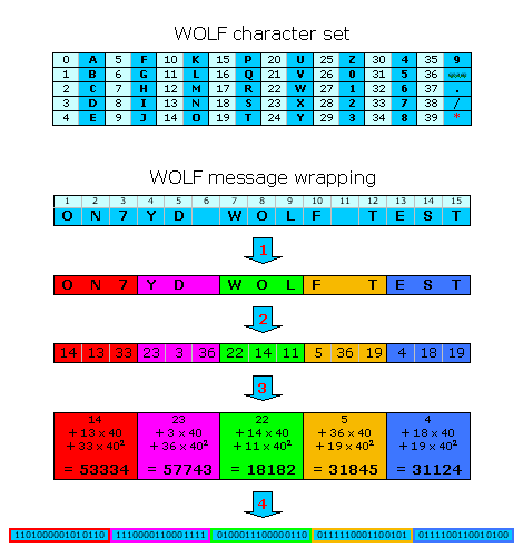Next the 15 character message is split up 5 groups of each 3 characters. If any possible combination of 3 characters is taken into account you have 64000 possible combinations (40 x 40 x 40). Thus each group fits into a 16 bit word (2¹⁶ = 65536), so the 5 groups (of each 3 characters) fit in a 80 bit data packet. Even though no real compression is done the 15 character message is wrapped efficiently into 80 bits.
As the next step a 1/6 rate FEC (Forward Error Correction) coding is applied. Forward Error Correction means that the transmitter is sending redundant data that can be used by the receiver to verify if the message is received correctly and correct eventual errors. The most simple method of FEC would be to repeat each character of the message a number of times. It is clear that the more times each character is repeated, or - more general - the more redundant data is transmitted, the better the error correction will be. In this case the 1/6 rate means that with each character of the original data 5 additional redundant characters are sent, what increases the 80 bit data to a 480 bit data stream (6 x 80). Of course WOLF is using a much more clever FEC coding than just repeating characters (in fact it is a rate 1/6 convolutional code that was considered for Galileo), but it would lead far beyond the purpose of this article to go into details.
Finaly after each "data" bit, a "reference" bit is added, increasing the stream to 960 bits long "frame". You can think of the signal as having a data channel and a reference channel. The reference stream is a long pseudo-random sequence that is known in advance by the receiver. Its purpose is to enable recovery of carrier frequency and phase, bit timing, and message timing, even when the signal is very weak.
At 10 bit per second it takes 96 seconds to transmit the 960 bits frame. It may look wasteful to blow up a 80 bits message to 960 bits, especially if half of is occupied by the reference channel that contains no information. At this moment the purpose of the reference channel is to enable recovery of carrier frequency and phase, bit timing and message timing, even when the signal is very weak. Future versions of WOLF might use it also for accurate path characterization.
If the signal is strong enough it will be instantly decoded correctly and the transmitted message will show up after it is transmitted once (96 seconds). But what happens if the signal is to weak to be decoded correctly at once ?
That is where the reference stream is used. It is mentioned above that the 15 character message is wrapped into 80 data bits and then 80 reference bits are added. The total energy of the (pseudo-random) reference stream is equal to that of the data stream and is thus 80 times (or 19dB) stronger than the energy of a single data bit. So even if the individual data bits are far below the decoding level the reference stream can still be used to determine the frequency and timing of the signal, and then estimate the phase with good accuracy. This information is used to try to demodulate the datastream, even if the individual databits are to weak to be decoded. Then the results of several frames can be added together, until the signal-to-noise ratio is good enough to decode the message.

6.3. Running WOLF
The original WOLF software developed by KK7KA runs under DOS (or in a Windows DOS-box) and it takes a WAV file as source (not soundcard input). The software can be launched with a number of command line options, allowing to select the center frequency, activate a noise blanker, add noise (for test purposes) etc.
The software output is :

WOLF returns a number of parameters followed by the decoded (or attempted decode) message :

t : elapsed time since start [seconds]

f : frequency offset [Hz] (frequency of the detected signal relative to the excpected frequency)

pm : power of best sync match [arbitrary units, linear]

jm : offset of sync pattern at best match [0 to 479]

q : SNR of the reference channel (1. value) and data channel (2. value) [dB]. Values above -5 (for data) should give correct decoding.

A complete frame takes 96 seconds and thus WOLF will try to decode every 96 seconds, with one exception. During the first frame WOLF will do 3 "quick attemps" to decode the signal, after 24, 48 and 96 seconds, based on a partial frame. If the signal is strong enough decodation might be successful already after these first attemps. During this first attempts some of the given parameters are different :

a : phase of the carrier relative to the start [radiants, -pi/2 to +pi/2]

dp : power of the detected carrier [dB relative, normalized to the length of the record]

ci : bit phase of the detected sync [1/80 second units, 0 to 15]

cj : offset of the sync pattern [0 to 479]

As you can see from the above example of WOLF reception the decoded message is complete garbage until all the sudden (at t: 384) it appears 100% correct. At first glance this might look strange and one would expect that the different characters of the message are gradually falling into place as WOLF can use more and more frames. But this effect can be explained by the fact that adding error correction (such as FEC) will improve decoding when the signal exceeds a certain level but at the other hand will make things worse below that level. With WOLF this threshold region (between no copy and perfect copy) is only 1dB. So sometimes you might see partial copy for 1 (or 2) lines.
As mentioned WOLF should perform correct decoding at an SNR (data channel) of -5dB or better. As can be seen in the example above the SNR gets better as more frames are received. Within certain limits one can use this increase in SNR values to predict the correct decoding when the signal (transmitter power) is reduced, assuming propagation and noise do not change. But be aware that the relation is worse than linear, since the sync recovery is less accurate at weaker signals.
Keeping in mind the threshold level of -5dB one would expect that decoding will be OK at t=576 if the signal level is decreased by 3dB and at t=1056 if the signal level is deceased by 6dB. The screenshots below show that the assumption is correct for the -3dB signal. But at the -6dB level decoding is correct only at t=1344 (3 frames later than predicted), what confirmes the worse than linear behaviour.

DL4YHF, Wolf B�scher (nomen est omen), developed a Windows based Graphic User Interface (GUI) for the WOLF software, including the decoding of signals direct from the soundcard and a QSO mode. This makes the reception and transmission of WOLF signals much more convenient.

6.4. Performance
Stewart Nelson, KK7KA, states :
"I am not aware of any objective tests of QRSS (where operators are presented with messages unknown to them, and the probability of correct decode is measured). However, it appears that the useful threshold of WOLF is similar to that of QRSS-60. Under such conditions, WOLF typically needs about 15 minutes for successful decode. Depending on message content, QRSS would be 6 to 10 times slower."

6.5. More WOLF
More information about WOLF can be found at :

7. Nihil novum sub sole

There is nothing new under the sun. Andr�, N4ICK, sent me a copy of an article that was published in RCA review of March 1966, titled "Low-power long-range digital communications system".
Some RCA engineers designed and tested a extremely narrow bandwidth communication system at a frequency near 15MHz. Based on receiver stability (1x10^-7) and ionospheric Doppler shift they came to a bandwidth of 1Hz. They wanted to use a small portable 100mW TX run from a 9V battery having a frequency stability of only 1x10^-6 what is insufficient to achieve a 1Hz bandwidth. Therefore 2 measures were taken :

The TX was swept over a 20Hz range every 20 seconds, to ensure that it would cross the RX passband even if the TX drifted +/- 10Hz away.
The RX had 3 sets of passband filters, each 17Hz apart. This allowed receptions even at a drift up to +/- 30Hz.

The disadvantage of all this measures is that the bite rate was reduced to 3 bits per minute. As 5 bit characters were used the data rate was 0.6 characters per minute. The block diagram of the RX is given at the left. It is based on a commercial receiver with a 500kHz IF output. This IF was converted to 20kHz and then filtered using a set of 6 crystal filters in the range of 19981Hz to 20017Hz.

At the right you can see the 100mW portable transmitter. As mentioned before the main problem was achieving the required frequency stability. This was done by keeping the crystal oscillator at a contant temperature ... using the human body as thermostate. The crystal oscillator was put in a small metal box (in the red ellipse), connected to the TX via a couple of wires. To keep the temperature stable the operator had to keep the oscillator in his armpit !
The tests showed that this way the SNR could be improved by about 40dB compared to conventional communication.

8. Available software

8.1. Spectran

Function	:	DSP receiving software
Operating system	:	Windows 95/98
Author(s)	:	A. di Bene (I2PHD) and V. De Tomasi (IK2CZL)
Description	:	This program allows extreme narrowband reception of weak signals. A lot of option, but they require some experience to use them proper.
Status	:	Freeware
Web page	:	here
Download	:	version 2

8.2. EasyGram

Function	:	DSP receiving software
Operating system	:	Windows 95 and up
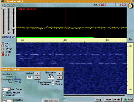
Author(s)	:	P. Maly (OK1FIG)
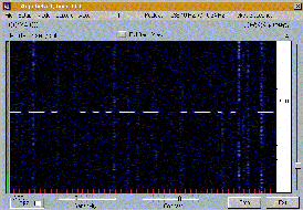
Description	:	This program extends possibilities of well-known Spectrogram with some new useful features. It enables to define the scrolling area to any size, it can save screen shots in defined time periods (useful overnight), it enables to browse the saved pictures easily. All the settings can be saved to named profiles.
Status	:	Freeware
Web page	:	here

8.3. Argo

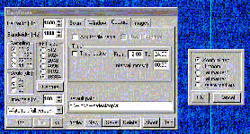
Function	:	DSP receiving software
Operating system	:	Windows 95 and up
Author(s)	:	A. di Bene (I2PHD) and V. De Tomasi (IK2CZL)
Description	:	Especially developed for reception of QRSS signals at 3 sec./dot and 10 sec./dot. Easy to use, since only very few parameters have to be set.
Status	:	Freeware
Web page	:	here
Download	:	beta 1, build 113

8.4. Spectrum Lab

Function	:	DSP receiving software
Operating system	:	Windows 95 and up
Author(s)	:	W. B�scher (DL4YHF)
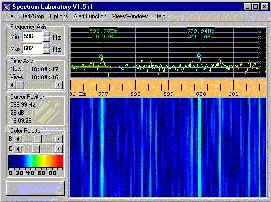
Description	:	Spectrum Lab incorporates a amazing number of features in a single program. Besides the 'standard' DSP rceiving window you can use it as a terminal for PSK, RTYY etc... and it will even allow you to decode the DCF77 signal and set your PC clock to it.
Status	:	Freeware
Web page	:	here
Download	:	here

8.5. Crunch

Function	:	DSP receiving software
Operating system	:	DOS
Author(s)	:	B. de Carle (VE2IQ)
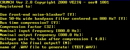
Description	:	A completely different approach to 'decode' QRSS transmissions is made by VE2IQ. With crunch the incoming audio signal is recorded as a WAV-file, either using the soundcard or VE2IQ's Sigma-Delta DSP board. Afterward the file is filtered and 'speeded up' to bring the QRSS signal to normal speed CW, audible via the soundcard.
Status	:	Freeware
Web page	:
Download	:	here

8.6. QRS

Function	:	QRSS and DFCW transmitting software
Operating system	:	Windows 3.11 and up
Author(s)	:	R. Strobbe (ON7YD)
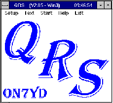
Description	:	This program is primarily intended to be used for QRSS and DFCW but has also some normal CW facilities. Keying of the transmitter and frequency shifting (for DFCW) is done via the serial or parallel port, using a very simple interface. Various options are available, including QSK and fast CW identification in QRSS and DFCW modes. In 'QSO mode' the program is optimized to share the screen with receiving software. Version 3.17 is Win3 compatible but will not support the parallel port under WinNT, Win2000, WinXP etc. Version 4.02 has full support of the parallel port but requires at least Win98.
Status	:	Freeware
Web page	:	here
Download	:	version 3.17 : here version 4.06 : here

8.7. Jason

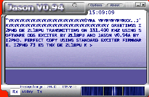
Function	:	Jason transmitting and receiving software
Operating system	:	Windows 98 and up
Author(s)	:	A. di Bene (I2PHD)
Description	:	a keyboard-to-keyboard communication program, tailored for very low S/N ratios, based on the IFK technique, using only 4 Hz bandwidth.
Status	:	Freeware
Web page	:	here
Download	:	here

8.8. WOLF

Function	:	software to generate and decode WOLF audio files
Operating system	:	DOS
Author(s)	:	S. Nelson (KK7KA)
Description	:	software to generate and decode WOLF audio files. Not suited for real time operation (see WOLF GUI for that)
Status	:	Freeware
Web page	:	here
Download	:	here

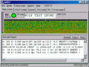
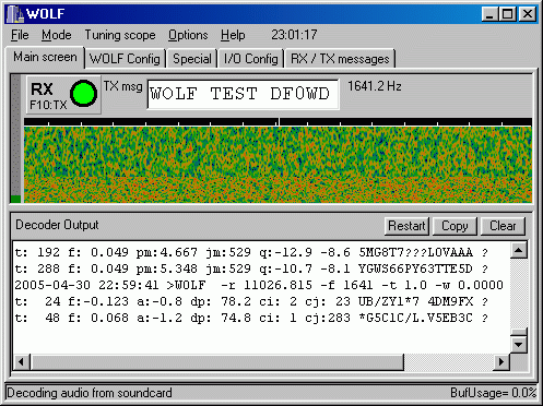
Function	:	GUI (graphic user interface) for KK7KA's WOLF software
Operating system	:	Windows 98 and up
Author(s)	:	W. B�scher (DL4YHF)
Description	:	GUI for real time generation and decoding WOLF signals
Status	:	Freeware
Web page	:	here
Download	:	here

8.10. Alternative downloading (mirror site)

Most of the above software (and a lot of other stuff) can also be downloaded from the NL9222 site.

9. Operating practice

Operating QRSS and DFCW is rather simple, just a few 'specialities' :

The (unofficial) QRSS/DFCW segment is 137600Hz - 137800Hz, most activity is between 137700Hz and 137750Hz
You need a stable TX : long term stability of 5Hz is an absolute minimum, 1Hz or better is recommended (for dotlengths in excess of 10 seconds stability should at least 1Hz, recommended 0.1Hz or better)
Keep your CQ's short : eg. CQ G3XXX K not CQ CQ CQ G3XXX G3XXX G3XXX PSE K
The report system is the TMO system (similar to EME) :
- T = signal traces seen but not good enough for a QSO
- M = weak signal but good enough for a QSO
- O = perfect copy
For intra-continental QSO's (eg. within Europe) :
- a dot length of 3 seconds is recommended, eventually 10 seconds if weak signals are expected
- for DFCW a shift of 2 to 5Hz (with 'dash' being the higher frequency) and a key gap of about 1/3 of the dotlength is recommended
For inter-continental (DX) tests :
- dot lengths up to 120 seconds are common
- for DFCW a shift of 0.1 to 0.5Hz (with 'dash' being the higher frequency) is recommended
During a QSO (once you are sure that both stations have the calls OK) you can use the suffixes instead of complete calls.
If you see the end of a QSO and you want to contact one of the stations you can start calling this station while the previous QSO is going on, just call on another frequency.
If replying to a CQ it is recommended to call NOT exactly on the frequency of the other station, this will avoid QRM in case more than 1 station is responding.
Due to the slow 'transmission rate' it is recommended to limit the QSO to exchange of callsigns and reports, especially if you are located close to another radioamateur that is active in this mode (one strong signal can 'block' the entire QRSS segment).