How important is a low VSWR
It is the
generally
accepted view amongst the more knowledgeable, that a low VSWR is
unimportant
when considering which antenna to put up.
I do not of
course include
resonant antennas such as beams or vertical’s that are designed to
provide a
good match to coaxial cable. Walt
Maxwell in his book reflections states, “too low a SWR can kill you”,
this
dramatic statement does not imply that we will shuffle off this mortal
coil
when the meter drops to 1:1, but refers to how a good antenna can
become no
more than a dummy load if we pursue the holy grail of a 1:1 VSWR
reading
without considering the implications.
You will
forgive me I hope,
if I repeat the words of many who have gone before, in saying it is
very
difficult to find a better and more versatile antenna than a reasonable
length
doublet fed with open wire feeder all the way back to the transmitter. The difficulty with such an antenna is that
we need a magic box to bridge the gap between the end of that open wire
feeder
and the ubiquitous SO239 socket on the back of almost every transceiver.
This is the
crux of the
problem; we must separate the antenna where the object is to provide an
efficient radiator preferably in some desired direction, from the
matching
which is the task of transferring the power from the transmitter to the
antenna
with as little loss as possible and a correct match for the PA.
In spite of all
the hype
that we hear on the amateur bands there is very little to choose
between the
various popular designs, if height and length are of the same order. For
any single wire antenna the
radiation pattern depends on its length in wavelengths and height above
ground. The main exception is the “V” inverted or
otherwise, because of it having a vertical component
to its radiation, some low angle radiation is gained at the expense of
some of
the normal horizontal pattern.
The same cannot
be said of
methods of feeding the antenna; I will show that some methods can lose
a very
large proportion of the transmitters output, and at the same time
showing a
very low VSWR. In fact it is a general rule that the more efficient an
antenna /
feeder combination, the more difficult it is to find a good match.
Since this
is the opposite to what we might intuitively believe, it is worthy of a
more
detailed explanation.
The lowest VSWR
is obtained
with a dummy load! However a length of corroded low quality coax makes
an
excellent dummy load. This is where a low VSWR reading should not be
regarded
as a sign that all is well, but rather should be treated with
suspicion, even
when using a resonant antenna such as a half wave dipole where we would
expect
to see a low reading, moving the transmit frequency away from the
resonant
frequency the reading should rise steeply, if it lingers near the
bottom of the
scale be suspicious!
VSWR and feeder attenuation
The VSWR at the
antenna
feed point is frequently impossible to measure, but can give an
indication of
whether a design is behaving as expected.
If we know the
matched loss
of the feeder and the VSWR at the bottom then it is possible to
calculate the
probable VSWR at the antenna end.
If we set (VF
+
VR) = 1 then since (VF
+ VR) / (VF – VR)
= VSWR
then (VF – VR) = (1
/ VSWR),
since
VF = 1
– VR and VR
= 1 – VF
2VF = 1 + (1 / VSWR)
and
2 VR = 1 – (1 / VSWR)
The forward
part of the
wave at the bottom of the feeder is: -
VFG = 0.5 + (1/(2*VSWR))
and
the reflected part is: -
VRG = 0.5 – (1(2*VSWR))
You will note
that whatever
the value of VSWR, when added together these two equations always add
up to 1
as we initially defined. These are the
relative amplitudes of the forward and reverse waves for that value of
VSWR at
the generator. As we move towards the
load, the amplitude of the forward wave reduces due to the feeder loss
and the
amplitude of the reflected wave increases since we are moving closer to
it’s
source with less loss.
The factor “M”
by which the
reflected wave must be multiplied and the forward wave divided can be
obtained
from the loss figure for the length of feeder used.
M = 10(dB/20)
(where dB is the loss in dB for the
length of
feeder)
(dB is divided by 20 because these are
voltage
ratio’s)
we can now
evaluate
expressions for the relative amplitudes of the forward and reflected
waves: -
VFL =
VFG / M
and VRL = VRG * M
The value of
VSWR at the
load end of the feeder is: -
VSWRL = VFL
+ VRL
VFL
- VRL
We can if we
wish use this
computed value of the load VSWR and the calculated figure for the
matched line
loss to calculate the actual feeder loss in the next section.
Actual feeder attenuation under VSWR conditions
If we
know (whether calculated or measured) the feed impedance of the antenna
and the matched line loss of the feeder, we can calculate the actual
loss. As
before the relative amplitude of the forward and reflected waves can be
calculated from the VSWR at the load. The
actual voltage (VFL + VRL), which we previously
assigned the value of 1, can be calculated for an arbitrary load power
of 1watt hence V = (P* R)-2 for P = 1watt
and R = VSWR * Z0 VFL=(0.5+(1/(2*VSWRL)))
* (VSWRL * Z0)-2 VRL=(0.5–(1/(2*VSWR)))
* (VSWRL * Z0)-2 This
time however we must multiply the amplitude of the forward wave by M
and divide the amplitude of the reflected wave by M
“M = 10(dB/20) VRG=(0.5+(1/(2*VSWRL)))*(VSWRL*Z0)-2 /
M VFG
=(0.5– (1/(2*VSWR)))*(VSWRL*Z0)-2 *
M Power
is V2/ R
(where R is Z0)
. V2 = P * R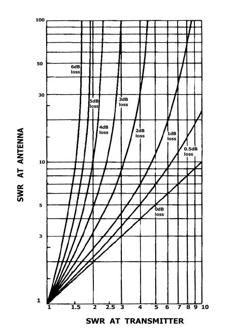
Fig.
1 curves of SWR at transmitter
against SWR
at load
Forward power is (0.5 + (1/(2*VSWRL)))
2 * VSWRL / M2
Reflected power
is (0.5 –
(1/(2*VSWR))) 2 *
VSWRL * M2
The power from
the
transmitter is Forward power - reflected power = Ptx
The power to
the load is
declared to be 1watt so the loss due to the feeder is: -
10*log10 (Ptx)
The accuracy of
these
figures depends on how accurately we can measure the VSWR at the
generator end
and how close
the actual
feeder loss is to the published value.
Looking at the Smith Chart
Phillip H.
Smith of Bell
Telephone Laboratories developed the Smith chart and an account was
published
in the American magazine ELECTRONICS in January 1939, subsequently an
improved
version appeared in January 1944.
This
simplified view of a Smith chart shows how the main axes of a normal
graph have been curved into circles and arcs. As is normal practice
with the Smith chart it has been normalised so that the characteristic
impedance Zo = 1, for Zo other than 1, all the figures are multiplied
by Zo. One rotation of the chart corresponds to a half wavelength of
transmission line; (the wavelength scale around the edge has been
omitted for clarity) to find the transforming effect of a transmission
line first you plot the load impedance on the chart, then draw a circle
centred the centre of the chart that passes through that point, this is
a circle of constant SWR. Moving clockwise around the chart for the
length of the line, remember one rotation is a half wavelength;
continuing to rotate adds one half wave for every complete rotation.
You can then read off the impedance that the generator will see from
the new position on the chart. Even in
these days of computers where transformations like this can be
calculated in much less than a second, the Smith chart is a powerful
visual tool. If the transmission line has loss, then reducing the
diameter of the SWR circle as it rotates can show this.