|
Page last updated: 23/11/2014 |
Time Domain Reflectometer
This Time Domain Reflectometer (TDR) is an add on to a standard oscilloscope, used to check the characteristics of feedlines. It is possible to detect damage to feedlines, short circuits, open circuits, water ingress, and furthermore identify exactly where the damage is. On one occasion I found damage at 1m interval over a 50m cable run up a mast, subsequently identified as over tightened zipties.
Design requirements
Simple design using readily available components.
Easy to build and set up.
Low power consumption suitable for battery operation.
A small and compact design.
Circuit description:
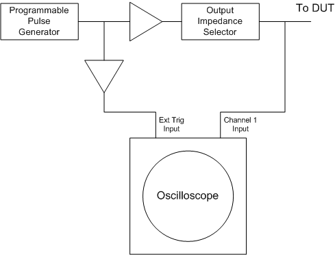
The block diagram below shows the oscilloscope TDR add-on in its most basic form
Based around a 74AC14 (hex inverter with schmitt trigger input) integrated circuit. One inverter (IC2d) is used as a pulse generator, the pulse width of between 5nS and 5uS selected by S1. The remaining inverters used as buffer / driver, IC2a,b,c, & f in parallel providing drive for the main output to the device under test (DUT) and oscilloscope main input, whilst IC2e to the external trigger input of the oscilloscope. The output impedance of either 50, 75, 100, 150, 300, 600 ohms is selected by S2.
Description of circuit in operation:
![]()
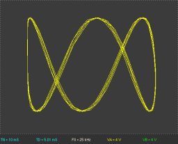
The leading edge of a pulse triggers the oscilloscope to begin a new sweep, this pulse also introduced into the cable to be tested. Now assuming the output impedance of the TDR, cable to be tested, and the load at the end of the cable, are all equal then the oscilloscope will show the trailing edge of the outgoing pulse followed by a flat line.
| If however the end of the cable under test instead of being terminated by a load is left un terminated then the pulse will be reflected back along the cable, and can be observed on the oscilloscope trace a short period of time after the outgoing pulse as a second positive going pulse. | 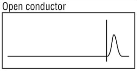 |
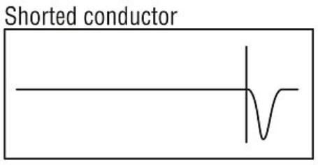
| Alternatively If the end of the cable under test instead of being terminated by a load is shorted then the pulse will be reflected back along the cable, and can be observed on the oscilloscope trace a short period of time after the outgoing pulse as a second negative going pulse. |
 |
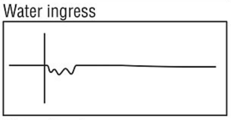
| Probably one of interest to those of us checking antenna feedlines is that of water ingress, in this instance ingress at an arbitrary point along a correctly terminated feedline. |
 |
Distance to fault can be relatively easily calculated. Electrical signals travels along a feedline at a little under the speed of light, there is the dielectric constant of the feedline (otherwise known as velocity factor) to be taken into consideration, and not to be forgotten in our case here it's a round trip time - there and back from the event in question. This however is not as daunting as it might first seem, the speed of light is a constant 299,792,458 m/s, manufacturers datasheets are available for most types of cable which will quote the velocity factor, then with a little maths we can calculate distance per unit of time - therefore the oscilloscopes horizontal timebase setting can be considered as distance per division as apposed to time per division
If we were looking at a length of RG59 cable, where
Speed of light = 299,792,458 m/s (~0.299m/nS) VF of RG59 = 0.83
0.299792458 * 0.83 / 2 = 0.12441387007 m/nS
And if the oscilloscope the horizontal timebase is set to 10nS/div each division then equates to ~1.25m
Other considerations:
Dead zone and range, or should I say dead zone vs range.
You may have noticed the outgoing pulse width is adjustable between 5nS and 5uS, the pulse width has a direct effect upon both the range and the dead zone of the TDR. Unfortunately whilst increasing the pulse width has the benefit of increasing the usable range of the TDR, it also has the detrimental effect of increasing the dead zone. It will therefore be found beneficial to use longest pulse widths when checking longer cable runs, but the shortest pulse widths with the shorter cable runs.
Sometimes it will be found advantageous to add an additional section of feedline of the same type being measured of defined length between the TDR and cable to be tested, where the dead zone will then exist only within the added section of feedline remembering to deduct the added cable length from the results.
Controls:
|
S1 Range |
Pulse length |
Fundermental frequency |
Blind spot |
Approximate range |
||
|
Twisted pair |
Coaxial |
Twisted pair |
Coaxial | |||
| 1 | 5 nS | 100 MHz | ||||
| 2 | 10 nS | 50 MHz | 4 m | 4 m | 250 m | |
| 3 | 20 nS | 25 MHz | ||||
| 4 | 50 nS | 10 MHz | 8 m | |||
| 5 | 100 nS | 5 MHz | 16 m | 17 m | ||
| 6 | 200 nS | 2,5 MHz | 30 m | 1.5 km | ||
| 7 | 500 nS | 1 MHz | ||||
| 8 | 1 uS | 500 kHz | 120 m | 133 m | 2 km | |
| 9 | 2 uS | 250 kHz | 192 m | 360 m | ||
| 10 | 5 uS | 100 kHz | 420 m | 600 m | ||
|
S2 Z out |
DUT impedance |
| 1 | 50 ohms |
| 2 | 75 ohms |
| 3 | 100 ohms |
| 4 | 150 ohms |
| 5 | 300 ohms |
| 6 | 600 ohms |
 Time Domain Reflectometer
schematic:
Time Domain Reflectometer
schematic:
 Time Domain Reflectometer
component placement / layout:
Time Domain Reflectometer
component placement / layout:
 Time Domain Reflectometer bottom
trace:
Time Domain Reflectometer bottom
trace:
 Time Domain Reflectometer parts listing:
 Time Domain
Reflectometer example trace patterns:
Time Domain
Reflectometer example trace patterns:
Original Files:
Further to the details of the pages above - the original CAD files created using EAGLE PCB Design software are included below, along with associated PDF files of both schematics and PCB layouts suitable for printing directly.
To use the original CAD files, they must be opened with EAGLE. Visit the CADsoft web site for more details, the software (including a freeware version), part libraries, tutorials, for EAGLE are available.
Time Domain Reflectometer schematic PDF
Time Domain Reflectometer PCB component placement / layout PDF
Time Domain Reflectometer PCB bottom trace PDF
Time Domain Reflectometer Eagle schematic
Time Domain Reflectometer Eagle board
Further reading & Reference material:
TDR Tutorial - Introduction to Time Domain Reflectometry
RADIODETECTION Application Note