How far can I get

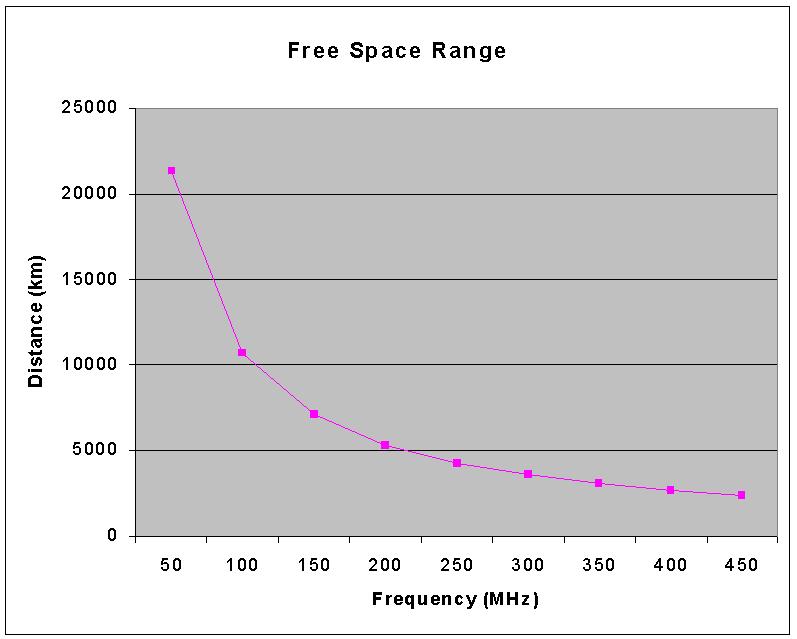
We all know that during a "lift" distances of 1000 kilometres or more are possible in the higher VHF and UHF bands, but how much range can be expected under "flat" conditions? Even before starting to transmit, we all have some idea of the range we might achieve based on our experience of radio systems within the bands. For example the FM Broadcast band is in the region of 100 MHz and anyone with an old style FM radio in their car knows it generally needs to have the channel changed every 30 to 40 Km. Newer radios with RDS do the re-tuning automatically. The Television band lies in the 600-800MHz region and the maximum range is usually about 50Km. So what is it that determines the range that can be achieved? An expression that is sometimes used in these bands (particularly at UHF) is that propagation is "line of sight". However, this tends not to be very useful – even as a rule of thumb. It’s easy to see why with a few simple calculations.

When professional engineers design radio systems they are usually interested in the range that can be achieved. It can be critical to get this right as a underestimate of only a few percent would mean huge additional costs with cell-phone systems which have many thousands of sites across the country. The first stage in all these calculations is to work out how much signal you can afford to loose along the path between the transmitter and receiver so that there is enough signal left to be readable. This is actually quite easy to work out. Let’s assume your receiver needs 0.5 microvolts for a readable signal. Using the familiar equation

We can calculate that 0.5 microvolts = 5x10^-15 Watts (a very small amount of power)

To make this easier to handle, we can turn it into decibels relative to 1 Watt, 10Log(5x10^-15)=-143dBW. If we assume that the aerial system has no gain (or loss), then this is the signal level that we need for acceptable reception. Now looking at the transmitter end, let’s assume that it runs 10 Watts (10dBW) and again that the aerial system has no gain so that the Effective Radiated Power is 10dBW. In this case, we can tolerate a loss of 153dB (the difference between 10dBW and –143dBW). This loss is sometimes called the Basic Transmission Loss.

If we imagine our path is actually line-of-sight (i.e. from the transmitting aerial we can see the receiving aerial), we can work out how far we can communicate using the Free Space Path Loss Equation which is:

Loss(dB)=32.4+20Log(d)+20Log(f)

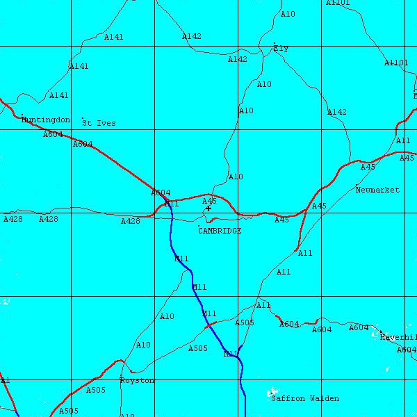
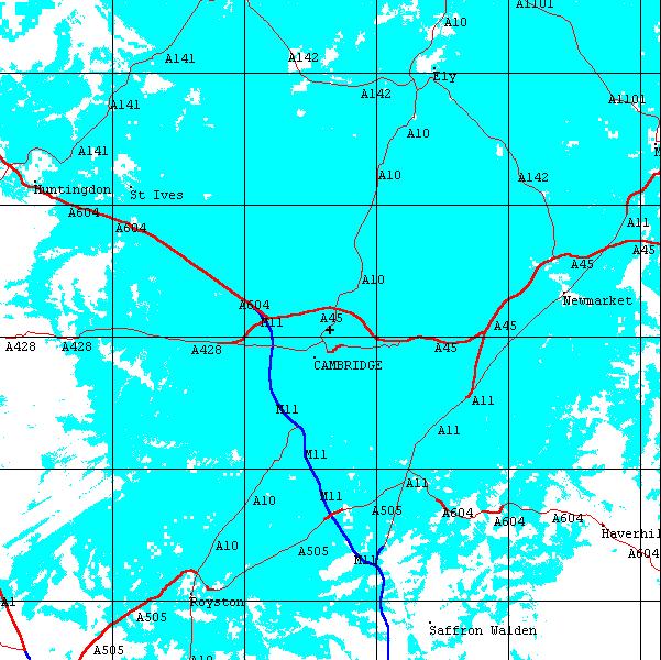
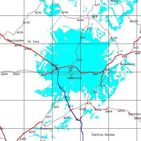
d is the distance in kilometres and f is the frequency in MHz. A bit of rearranging and calculating and we can construct the following range graph.

Judging by this graph, on 6 metres (50MHz) you might expect a range of 22,000 kilometres and on 2 metres (145MHz) a range of around 7,000 kilometres. These distances would be accurate in Space but the actual ranges you might achieve here on Earth under flat conditions are much less, so the conclusion is that there are some other losses involved that we have not accounted for. These losses come from a variety of sources but the two major ones are blocking of the signals due to terrain – the signals don’t bend around hills very well, and blocking of the signal due to trees and buildings. The other major factor is that as the earth is not flat, after the horizon is reached the curvature of the earth itself gets in the way. Now we are into some much more complex calculations to work out the range. Professional engineers use a variety of techniques to estimate the range taking into account the various obstructions we have identified. The most commonly used techniques calculate the diffraction losses over the obstructions. This can be very laborious as to calculate the range in any one direction, the calculations need to be done for all the points along the path. Fortunately, computer programs take the hard work out of this. Below are three coverage predictions from a sophisticated software propagation-modeling package. It uses terrain heights accurate to 1 metre, every 50 metres along each path. It also has details of other obstructions in the area such as houses and trees. To generate these predictions I have selected a site somewhere in Cambridge and simulated a transmitter there with a vertical dipole aerial 10 metres above the ground. Using the figures above, the light blue colour show where we would expect to get coverage with a probability of 90%. The grid on the plots is 10km. On 6 metres (50 MHz) virtually the whole area is covered. Moving to 2 metres (145MHz), there are some white patches indicating areas that are not covered to the standard we specified. On 70 centimetres (435MHz), the range has dropped dramatically with coverage only reaching about 10 to 15 kilometres in each direction.

50MHz Range

145MHz Range

432MHz Range

Considering the modeling problems presented by the complexities of the environment, it is perhaps surprising that professional engineers have developed some fairly simple formulae for predicting average ranges that don’t need any terrain information. The best know of these was proposed by Hata. His formula allows a range to be calculated from frequencies between 150 and 1000MHz in a variety of situations. Unfortunately, it is not too much use for radio amateurs as the minimum aerial height that can be modeled is 30 metres.

What is clear is that as a rule-of-thumb range drops with frequency all other things being equal. But that’s not the whole story. In built-up areas, the higher frequencies tend to reflect better and can penetrate buildings better as the shorter wavelengths can enter through windows. This effect is often quite marked in road tunnels where 2 metres fades quickly whereas 70cm goes on much further. So in built-up areas, higher frequencies may prove more effective. Another factor to consider is that at the higher frequencies, due to the shorter wave-length, aerials become smaller and so for a given physical size of aerial, more gain can be achieved countering the increased losses.