What is "CalcEd" ?
On the first glance, CalcEd looks like a simple text editor. It handles large
files (>64k) and rich text files (*.RTF). But its main purpose is: CALCULATING
! You can use it for step-by-step calculations, and save all steps in a simple
textfile.
This information is copied from CalcEd's manual, it may be quite outdated
(you will find a more up-to-date manual in the zipped archive, along with
the executable).
You can download CalcEd from this site (see end of
this document).
Basic operation as calculator
To calculate a formula, simply enter it in a new text line like this:
1+2
Then, with the cursor still in the line of the formula, press F7 (or use
the "Calculate" menu, or shift-ENTER to produce the next line). When a (normal)
formula is be calculated, the result is "printed" into the same text line
like this:
1+2 =: 3
The "= :" token (without the space) is a keyword, which shows CalcEd that
a line is a "formula" which must be re-calculated when you press F9 (to update
all results). Be careful not to use this token in "normal" text which shall
not be affected by F9 = "Re-Calculate All".
This is all you have to know to use CalcEd for simple calculations !
Examples: Resonant frequency of an L/C tank circuit (inductor and
capacitor)
1/(2*pi*sqrt(1.36mH*1nF)) =: 136474
1/((2*pi*136.5kHz)^2*1nF) =: 0.00135949
-
Notes
-
CalcEd accepts "technical" exponents (powers of ten like p="pico", n="Nano",
m="Milli", ... M="Mega" .
-
There must not be a space character between the number and the exponent,
no matter if mathematical ("1.23E-6") or technical ("1.23uF", see below)
.
-
Americans beware: "m" is NOT MEGA, it's milli ! 14 mHz is a strange frequency
for a ham radio transmitter ;-)
A physical dimension may be appended directly after a "technical" exponent,
like pF="picofarad", kOhm="kilo-ohm" etc. The physical dimensions are skipped,
you can use them for clarity. CalcEd will happily add apples and pears if
you want it to.
You can use the result from one calculation in the next calculation. The
underscore character (_) is the token for a variable which holds the last
result.
	1+1 =: 2

	_*_ =: 4

	_*_ =: 16

	_*_ =: 256

	_*_ =: 65536
The underscore as placeholder for the "last result is the easiest way to
do step-by-step calculations.
Numeric Variables and Functions
For better clarity, variables can be used. Variables always begin
with a capital letter (to tell them from built-in
functions):
R1 := 1+2+3 =: 6

	L1 := 1.36mH =: 0.00136

	C1 := 1.0nF =: 1e-09
Note: Unlike many programming languages, you don't have to declare a variable.
You just use it and it begins to exist !
To assign a new value to a variable, use the operator symbol ":=" in the
formula, and calculate it with F7 (or shift-return).
If you don't want to see the result in that line, enter the "at"-sign in
the first colum. The editor will see that this line contains some kind of
command, and that it's neither normal text nor a normal formula.
@X1 := 10
@X2 := 20
X1+X2 =: 30
Complex Numbers
Important about CalcEd (at least for its author) is, it calculates with
complex values. This helps a lot to calculate electric AC networks,
where its sometimes tricky to calculate the phase shift from inductors and
capacitors. Even the frequency response of a complex networks
can be calculated this way, without the necessity to solve linear equations
(see the "bandpass"-example in the CalcEd archive).
Complex values are noted as a sum of real and imaginary part.
Here we simply add two complex numbers (parenthesis just for clarity):
(1 + j*2) + (2+3*j) =: 3 + j* 5
Many (but not all) of CalcEd's internal functions support complex values:
sqrt(-2) =: 8.66311e-17 + j*1.41421

	_*_ =: -2 + j*2.4503e-16
(Note the rounding problem!)
sqrt(1+j) =: 1.09868 + j*0.45509

	_*_ =: 1 + j* 1
exp(1) =: 2.71828

	exp(j) =: 0.540302 + j*0.841471

	exp(1+j) =: Nur imaginaerer Exponent zur Basis e.
-
Notes:
-
e is the "natural number" 2.718... , and exp(x) is "e power x" .
The error messages may have been translated into English by the time you
read this.
Parallel resistors (or impedances) in electric circuits
Because connecting two resistors in parallel is a common task in the electronic
business, there is a special "parallel" operator in CalcEd (the two
parallel "pipes").
-
Note:
-
"C" programmers please take care, || is not the "boolean or" !
The operator "^" means "power" (A^2 is "A squared", not "A EXOR 2" as in
"C").
Examples:
R1 || R2 =: 40
30 || 30 || 30 =: 10
This also works for complex values:
(1+2*j)||(3+4*j) =: 0.769231 + j*1.34615

	(3+3j)||(3+3j)||(3+3j) =: 1 + j* 1
Built-in functions and other syntax elements
A list of all supported operators and functions is in the manual, which is
part of the downloadable archive. A short reference
of the built-in functions can be displayed through CalcEd's 'Help'-menu.
Outside the body of a self-defined function, commands must be preceeded with
the ampersand character ("at"-sign, @), so CalcEd can see that a line contains
a command, function call, or similar.
You can type 'normal' text between the calculations for documentation (or
remarks). This may change in a future version(*) of CalcEd: Within sections
of classic program code (with loops, branches, etc) it will be necessary
to put remarks into comment sections like the following:
/* This is, and will ever be, a comment */

	// This is also a comment, C++ style

	REM This is a comment too, stoneage BASIC style
(*) In fact, there is a CalcEd-variant with a tiny programming language built
inside. But it's too early to be spread around..
Function plotter
There is a simple function plotter in CalcEd which can be invoked with this
command:
@plot(<feeder>:=<start_value>..<end_value>,<function1>[,<function2>]
[,...] )
-
where
-
<feeder> is the name of a variable for the X-axis (often "X"),
<start_value> is the first value (for the start of the X-axis),
<end_value> is the last value (for the end of the X-axis)
<function1> is the name or the definition of the first function to
be plotted (or a 'calculated' variable like "Y"),
<function2>..<function8> are optional functions which can be
plotted into the same diagram window.
-
Examples:
-
@plot(X:=-pi..pi,sin(X),cos(X))
@plot(X:=0..400,sin(X)/(X+10))
Note: During the execution of the "plot" command, the whole document is
calculated over and over, so it takes some time. Assignments to
<feeder> (here: X) are suppressed during the calculation.
A more sophisticated example for the plotter can be found in the file
"coupled_bandpass.txt" . It calculates and plots the amplitude- and phase
response as function of frequency for a bandpass made of loosely coupled
tank circuits: The command...
@plot(F:=135kHz..138kHz,20*log(A2),ang(U2)*180/pi)
... opened this plot window with the amplitude- and phase response of a simulated
bandpass filter:
Files contained in the 'Calc_Ed' archive (calc_ed.zip)
Of course, the archive contains the windows executable (see
'download' link further below). No installation required
- just unzip into a directory of your choice . It's up to you to keep the
following files (besides the executable), or to trash them immediately. They
are not required for the 'normal' operation of CalcEd.exe .
CalcEd is distributed along with a few (text-)files which are actually sets
of formulas, including...
-
pi_filter_designer.txt : Simple Pi filter designer (RF bandpass + impedance
matcher).
Calculates the values for a PI filter (with two capacitors and one inductor)
for a given frequency, input- and output impedance, and Q factor; then simulates
it, and plots the input impedance and 'gain' over an adjustable frequency
range. Very handy for RF circuit design, especially for 'QRP homebrew' where
such PI filters are used between the power amplifier and the antenna output.
The PI filter removes harmonics, and also transforms the output impedance
of the amplifier (tube or transistor) to the antenna- or coax cable impedance
(which is typically 50 Ohms). A part of the PI filter's input capacitor can
be the transistor's (or tube's) output capacitance. If the calculated "C"
values for the filter are too small, try again with a larger "Q" value for
the design.
-
lc_resonant_transformer.txt : Simple L/C "up" transformer (low impedance
input, high impedance output) which is sometimes used in very simple,
low-voltage, narrow-band amplifiers with bipolar transistors (as an even
simpler, and low-loss, alternative to the Pi-filter).
-
lc_resonant_transformer_hi_to_low_z.txt : Similar as the previous, but for
an impedance "down"-converter (high impedance in, low impedance out, also
acts as a lowpass filter). In contrast to the previous file, the input for
this calculator are only the frequency, input, and output impedance (nothing
else, the program doesn't care for 'standard inductor values' etc).
-
quarterwave_coax_resonator.txt : A rather exotic project. It simulates a
quarterwave resonator, using lossy coaxial cable (loss estimated from skin
depth, and copper conductivity. Dielectric losses were ignored).
-
coupled_bandpass.txt : Simulates a preselector using 'two loosely coupled
resonators', including the losses (which some others decided to ignore, which
is a bad idea). The plotted graph shown in the previous chapter was calculated
with this file ("program"). The author used such a bandpass as 'preselector'
in a homebrew narrow-band longwave receiver. The output ("Ro") was actually
the gate of a field effect transistor.
-
microstripline.txt : Calculates the impedance of a microstripline, using
the PCB trace's height, width, copper thickness, and the dielectric constant
of the board material (Epsilon r). This was just a test to compare different
formulas (to calculate microstripline impedances) found on the net; with
the result that they gave *very* different results !
-
moontrak_wb7cci.bas : A stoneage 'Basic' program (modified to run in CalcEd)
to track the moon's azimuth and elevation for any given date and geographic
location. Credits to WB7CCI who wrote the original code, and G3RWL who converted
it to 'Disc Basic' and published it somewhere (don't remember where exactly).
If you're serious into EME (Earth-Moon-Earth communication), you will certainly
use a different software to point your antenna to the moon, though ;-)
-
sun_position.txt : You guessed it ;-)
-
fft_windows.txt : Plots some common FFT windowing functions.
-
vswr_vs_load_impedance.txt : Calculates and plots VSWR (Voltage Standing Wave Ratio) and return loss versus load impedance.
        Zsource := 50         ;  source impedance [Ohm, usually real]
        Zload   := 50 + j*20  ;  load impedance [Ohm, possibly complex]
        Gamma := (Zload-Zsource)/(Zload+Zsource)
        VSWR := ( 1 + abs(Gamma) ) / ( 1 - abs(Gamma) )
        ReturnLoss_dB := -20 * log((VSWR-1) / (VSWR+1) )
        ; Show results in numeric form:
        VSWR           =: 1.48792
        ReturnLoss_dB  =: 14.1497
        ; Plot VSWR and Return Loss (in dB) versus different load impedances :
        @plot(Zload:=15 .. 150, VSWR, ReturnLoss_dB)
Output for various load imdedances (in Ohms, on the horizontal scale) for a 50 Ohm source:
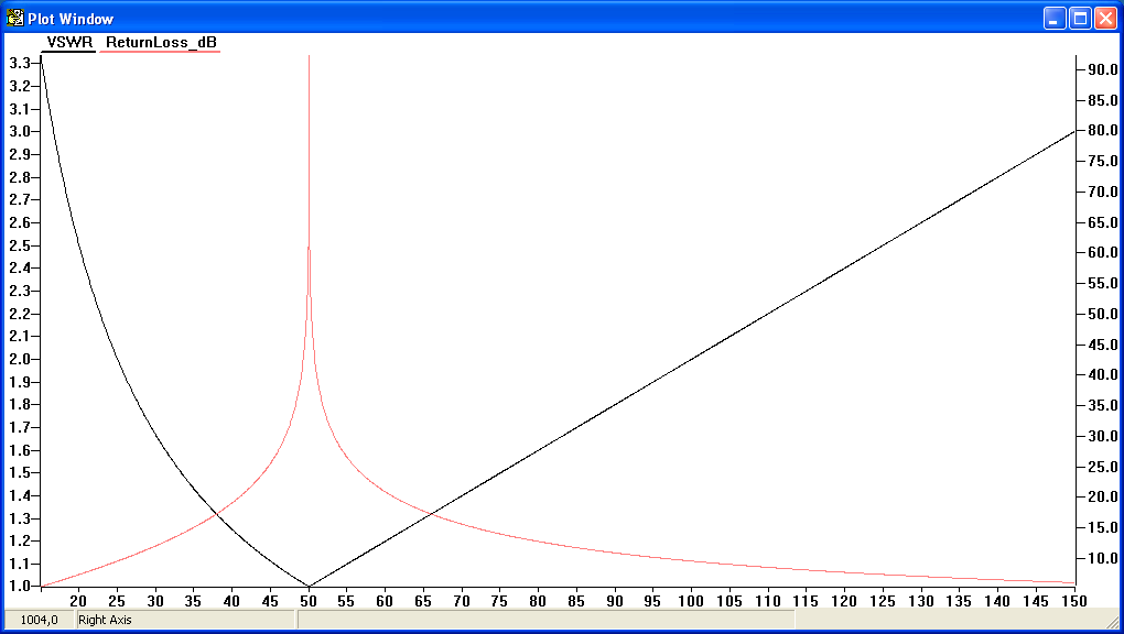
CalcEd's "plot window". Click on image to magnify.
Disclaimer and
Download
I hate this legal stuff, but here it comes again:
The author provides this software "AS IS" without warranty of any kind, either
expressed or implied, including, but not limited to, the implied warranties
of merchantability and fitness for a particular purpose.
The entire risk as to the quality and performance is with you. In no event
unless required by applicable law will the author and/or any other party
who may modify and/or redistribute this software be liable to you for damages,
including any lost profits, lost monies, or other special, incidental or
consequential damages arising out of the use or inability to use this package,
or for any claim by any other party.
This program is still "under construction", and there are certainly a number
of bugs lurking in the code. The entire risk is with you. You may find udates
at the DL4YHF website (search for DL4YHF CalcEd) . User feedback is
welcome !
If you have a good reason why you need the ugly sourcecodes, please
ask (for non-profit use only!). CalcEd is written in "pure C" without using
a toolbox (neither MFC,VCL,CLX or whatever).
Download CalcEd (executable and manual) from here:
calc_ed.zip
To install, just unpack the executable and the manual from the zipped archive
into a directory of your choice. No extra DLL's are required in the current
version of CalcEd. At the moment, CalcEd runs under Win95-98-XP-7-8-10.
A Linux compilation may be available one fine day ;-)
Author: Wolfgang Buescher (DL4YHF). Mail: On my main website.
|