Tropospheric Scatter Propagation
Ian Roberts ZS6BTE *
Reprinted as
published in Radio ZS, December 1984
Introduction
During the last 20 years or
so, with the appearance of high power UHF amplifiers and low noise signal
amplifying devices, a wide-band propagation mode capable of conveying VHF
signals over distances of 800 km or more has become increasingly important in high
priority commercial and military links.
The mode is loosely referred
to in the industry as “tropo” or “tropo scatter”.
In recent years the pages of
Radio ZS have recorded interesting long distance VHF and UHF phenomena as noted
by local radio amateurs. It is evident, though, that many of the reports are
rendered “tongue in cheek”, without much understanding of the propagation
mechanism witnessed and it is commonplace to see E, sporadic E, F2, E/F2 backscatter, tropospheric
ducting and tropospheric scatter confused.
The first five modes depend
entirely upon solar radiation of the upper ionospheric layers for success, the
latter two have nothing to do with solar activity. Tropospheric ducting is a
freak occurrence involving inversions or peculiarities in the moisture content,
pressure, and temperature domains in the vicinity of the ground and hence may
be detected by antenna systems. The mode is obviously unpredictable.
Accordingly, with solar activity presently at a low level, the only long
distance mode left for the VHF enthusiast is tropo scatter. Radio amateurs,
with their unique talents and privileges, are in a particularly good position
to add greatly to the existing knowledge of tropo scatter.
Background and history of tropo scatter
Marconi described tests in
1933 at 550 MHz over a 270 km path between Rocca di
Papa,
In 1949 the
By 1953 Bell Telephone
Laboratories, primed by much theoretical speculation and increasing empirical
evidence put forth their “Polevault” VHF over the horizon communications
system.
Armstrong, in work previously
unreported, verified independently propagation at ranges up to 500 km.
The US Air Force, in about
1955, took the plunge and commissioned a link over hostile territory, thereby
obviating the need for numerous conventional line-of-sight links.
And that is where the mysteries
of tropo scatter propagation have been largely hidden, in classified material,
generally not available to the radio amateur. Additionally the precise
methodology of tropo scatter remains ill-understood even in professional
circles and most performance evaluations are based on empirical data collected
during field testing.
Concepts and Parameters
Various important parameters,
peculiar to the mode, need further examination.
The K-factor,
generally K4/3 radius of the earth.
Much as light passing through a prism refracts towards the denser medium, so a
VHF beam passing along the surface of the earth tends to refract along the
denser air at the surface to achieve a distance considerably more than the true
line-of-sight condition. This accounts for the fact that radar, operating for
example at L-band (1100 MHz), can “see” a target below the visible horizon
(which is itself below the physical horizon) Fig 1.
Fig. 1: Bending of antenna beam due to
refraction (True earth radius, a)
Typically K is described as
K4/3 at frequencies below about 1 GHz; meaning over the horizon propagation,
but under severe conditions may fall to below unity.
Generally, K =effective radio earth
radius/true earth radius and is greatly dependent on the surface refractivity
index of the terrain over which the VHF beam is passing. In
There is a non-correlation
1)
in the signals received by two adjacent antennas
from a dual polarisation transmitting site when the receiving antennas have
opposite polarisation, e.g., horizontal/vertical, Fig 2.
2)
in the signals received (same polarisation) by two
antennas spaced a finite distance apart, e.g.
100 wavelengths, Fig. 2.
3)
in the signals received (same polarisation) by two
antennas receiving signals widely separated in frequency, e.g. 10 MHz, Fig.2.
4)
in the signals received by two antennas with slightly
different beam headings, Fig.2.
Fig. 2:
Non-correlation between the signals received by two antennas with 1) opposite
polarisation 2) physical separation of 100 wavelengths 3) slightly different
beam headings 4) wide frequency separation
These characteristics are put
to good use in professional systems. For example, a tropo link with “quad
diversity” would often use parameters 1) and 2) and be capable of receiving
both horizontal and vertical polarisation on each of the two antennas spaced
apart as above. Each antenna, similarly, would transmit horizontal and vertical
polarisation on a common frequency.
FM is currently the preferred
mode. The various signals are combined at IF (pre-detection combination
diversity). Since the respective noise inputs add in random fashion and the
signals linearly, a higher signal to noise ratio is obtained. Typical signal to
noise ratios (with psophometric weighting) are plus 40 dB – good enough for a
good quality telephone line or medium speed data with error correction.
A representative tropo link
uses quad diversity, 27m parabolic antennas, 10 kW c.w. at 900 MHz, carries 132
FDM telephone channels, distance 500 km. A link of this nature would otherwise
require 10-15 line-of-sight microwave stations.
Geometry of Tropo Scatter Path
Fig.3: Geometry of Tropo Scatter Path
R is 4/3 earth radius (8446
km)
D is great circle path
distance
h1 and h2 respective antenna heights above sea
level
h11 and h12
height of radio horizons above
seal level
d1 and d2
great circle distance between radio horizons and respective antennas
The scatter angle Ө = Ө0 - Ө1
- Ө2 radians
where Ө0 = d/R
Ө1
= ((h1- h11)/d1
+ d1/2R)
Ө2
= ((h2- h12)/d2
+ d2/2R)
Typical scatter angles are up
to 4 degrees.
Each 1 degree increase in
scatter angle introduces an additional 10 dB path loss and high value scatter
angles are avoided in professional systems. This is easy when one can choose a
mountain top site.
In Fig. 3 the zone where the
beams intersect is called the scatter volume and the properties of this volume
define the quality of the scatter path.
Amateur application of tropo scatter
Inspection of a standard K4/3
path profile indicates that one may not expect a local radio horizon (d1 and
d2) of more than 30 km assuming 20 m antenna height and level
ground.
Under these conditions could
one expect a tropo scatter path to exist between
In order to address this
question it is necessary to calculate or estimate the following:
a)
distance
b)
scatter angle
c)
path loss
d)
system noise
temperature
e)
signal to noise ratio, which would give an indication of the
signal to be expected.
a) The distance is calculated
from the great circle path distance equation by assuming JHB to be the point of
departure and using the respective latitudes and longitudes. So d = 872 km
b) The Scatter angle
The take-off from the PE end
is particularly advantageous with the beam passing over the
So, retaining the nominal 30
km radio horizon at 20 m antenna in JHB and remembering to use the same units
in the equation: h1 in JHB about 2 km with horizon at 1.38 km (hills
south of Alberton) h2 in PE at 0.5 km with horizon at 0.48 km (60 km
out) then scatter angle:
= 872/8448 – ((2.0-1.38)/30 + 30/16896) –
((0.5-0.48)/60 + 60/16896)
= 0.0769 radians
Ө = 4.4
degrees
c) Path Loss
The median path loss LP consists
of three components, viz.
LP = LFS + LS
– 0.2(NS – 310) dB
LFS = free space path loss, 92.4+20log
dkm +20 log FGHz
where d =
distance in km, F = frequency in GHz
i.e. LFS = 125.18 dB
Ls = is the all year median scatter
loss normalized at a surface refractivity index NS 310
=
57 + 10log(0-1) + 10log(F/0.4)
=
81.96 dB
The factor NS in terms of C.C.I.R.
recommendations and is mapped globally. In
So LP = 213.14 dBi
(this is an EME - type
path loss).
d) System Noise temperature
TSYS = α(Tα) + To(1-α) + T1
+ Tm/gm-1
where α = transmission line coefficient as a factor, 0.8 for 1 dB loss
Tα = temperature of transmission line, k, equal to To for uncooled lines, (= 290k)
To = ambient temperature k, typically 290
T1 = temp of 1st RF amplifier
stage, 150k (preamp used)
Tm = temperature of 2nd RF
amplifier stage (the receiver 600k )
gm-1 = gain of stage T1 = 32 (15 dB)
(The terms were explained in reference 3)
So TSYS = about
460k
The receiver noise power ratio Pn consists
of the “pure” KTB noise modified to incorporate the receiver noise figure, i.e.
FkTB, where F is the receiver’s noise figure. If one assumes the receiver’s RF
stages to be T1 and Tm with
filter losses of 1 dB, then F1 is about 2 dB. In a bandwidth of 1000
Hz, Pn turns out to be -168 dBW
e) Signal to noise ratio
SNR =
Gt = gain of Tx antenna, dBi
(12.0)
Gr = gain of Rx antenna, dBi (12.0)
LP = tropospheric scatter path loss, dB (213.14)
Pn = noise power ratio of Rx =
10log FkTB, -169, k is Boltzman’s constant 1.38 x 10⁻²³ and B = 1000
Hz in CW, T= TSYS , F is Rx noise factor =
2
So SNR = 20+12+12-213.4-(-169)
= -0.40 dB
However, since an isotropic path was used about 5 dB
should be added to this. The ear should have no trouble tracking a beacon-like
signal at this sort of SNR, indeed it should be
continually audible with signal levels changing in sympathy with changes in the
surface refractivity index. For example, an increase in this quantity from 280
to 300 would reduce the path loss by 4 dB and increase the SNR accordingly.
General
As a matter of interest, the typical heights of the
scatter volume (assuming unobstructed paths) are listed below:
|
distance |
150 km |
300 m |
2000 m |
|
|
300 km |
600 m |
3000 m |
|
|
600 km |
3000 m |
20000 m |
The shorter paths are characterised by deep, fast
fading. Longer hops show a steadier path loss consistent with the median path
loss for that month. It is suggested (in classified literature) that the best
tropo conditions prevail during a hot, summer afternoon, while the worst
conditions occur during winter nights.
Much remains to be researched, or remains unreported.
For example, what is the effect of a thunderstorm on the scatter volume? What
happens when a tropospheric duct intercedes? Is the north/south path more
favourably propagated as in F2 /TEP propagation? ** See p.s. at end
of this article.
Numerous high power RF sources exist in
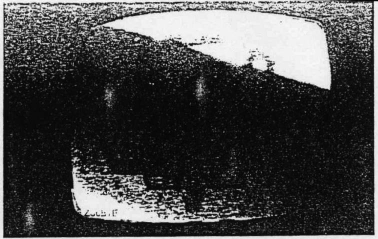
Tropospheric Scatter reception: the SABC’s Nelspruit ch. 24 TV transmitter received
over a scatter path of 270 km, the shadowing is typical of a camera with focal
plane shutter.
Conclusion
A method has been illustrated whereby VHF signals can
be propagated much further than the normal line-of-sight, point-to-point,
condition.
References
1) VHF-UHF Manual (RSGB)
2) Tropospheric Scatter (Point to Point Communications,
Feb; 1964)
3) System Noise Temperature and System Performance (Radio
ZS, Sept; 1982)
4) Radio Relay Systems (Thomson-CSF 1981)
* P.O. Box 32564, Glenstantia
0010
** p.s. added
1. Thundershowers in the scatter volume increase the
refractivity index and the S/N ratio by around 20 dB. Lightning bursts in that
volume further increase the S/N ratio 10 dB or so by providing a more solid reflection
sheet. The carrier frequency is much more dispersed, by as much as 100 Hz at
UHF under severe thunderstorm/unsettled weather conditions.
2. The north/south path does not show noticeable enhancement.
3. The effect of a tropospheric
duct remains untested.