It would also be useful to look at An Introduction to HF Propagation and the Ionosphere, where the history of ionospheric study and the physics involved are discussed.
VK2BLR received by ZL1BPU Feb 2004
(Click on image for full-sized view)
SBSpectrum is an important tool for the Radio Amateur, and was written by Peter Martinez G3PLX specifically for the analysis of radio signals. SBSpectrum dates from the days before PC sound cards (late 1990s), and yet remains today the best available software for radio carrier Doppler analysis.With a suitably stable transmission to monitor, and an equally stable SSB receiver, it is possible to measure very tiny frequency shifts in the received signal frequency that result from changes in the ionosphere. These changes occur because the propagation path is never static, and in some locations (especially near the poles) and some times of day, the apparent height at which signals are reflected changes quite markedly, leading to quite easily observable frequency shifts, known as 'Doppler shift', as the carrier frequency wavefront is compressed or expanded by reflection or refraction off moving objects, including the layers in the ionosphere. It is the rate of change of apparent height of the ionosphere which induces the frequency shift.
In addition, by monitoring a transmission over a long period of time (say 24 hours) you can also measure the signal strength, discover times of day when no propagation exists, and also determine when reception is focussed (direct or by stable refraction) or diffused (scatter, unstable refraction), and even determine which ionospheric layer is providing the path.
The secret weapon used for this analysis technique is the Narrow-Band Spectrogram. SBSpectrum is the supreme example. The Doppler shift which occurs generally does not exceed 1 part in 106 (1Hz per MHz), so the spectrogram used needs to have a span of 10Hz or better, and a resolution of better than 0.1Hz to be useful.
At this point it would be especially useful for the beginner to read the historically important paper Using Doppler DSP to Study HF Propagation, written by Peter G3PLX, and published in Radio Communications Magazine, May 1998.It would also be useful to look at An Introduction to HF Propagation and the Ionosphere, where the history of ionospheric study and the physics involved are discussed.
VK2BLR received by ZL1BPU Feb 2004
(Click on image for full-sized view)
SBSpectrum uses a Digital Signal Processing technique called the 'Fast Fourier Transform', to display a spectrogram, a graph of frequency versus time, with a third axis (brightness) representing signal strength. In the image above, the horizontal axis is local time (hours), and the vertical axis is frequency (Hz), with a total vertical width (span) of 5Hz. The resolution of the software at the setting used for the above recording is 256 samples over 5Hz or about 0.02Hz.Look closely at the image above (click on it for an expanded view). This is a recording of reception of a 2W transmission on 3600kHz from VK2BLR, received 2500km to the south-east of the transmitter. Even during daylight hours (1800 - 2100 local time) the signal was clearly detectable by SBSpectrum, although would not be heard by ear. Most (even experienced) Radio Amateurs would not expect to hear daytime transmissions on 80m from this distance, since during the day the D layer supposedly absorbs most of the signal before it reaches the upper ionosphere, and completes the job on its way back. However, the absorbtion is not always complete, and the sensitivity of the spectrogram technique allows even a puny 2W signal to be detected via its E-layer daytime reflection. The E layer is relatively stable, and shows little Doppler shift on the scale observed here.
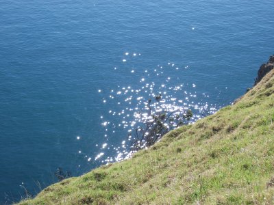
At about 2100 the D layer (at this frequency it absorbs but does not refract) stops absorbing completely, and the signal starts to be seen from various unfocussed higher scatter paths, and then reflected from the F-layer. At this time the effective height of the F layer is rising as ion density decreases (now after sunset midway between transmitter and receiver), and as the height is increasing, the reflected signal is low in frequency by several Hz, due to Doppler shift. There are short duration individual paths observed (the more defined dark areas), but much of the propagation is scattered due to the instability of the F layer - no one fixed reflective point, but many reflective points of short duration.These reflective points of short duration (scatter) can be easily pictured with an analogy. Imagine the F layer as the sea with small ripples and waves, reflecting sunlight back to the viewer, as in the picture on the right. There's not one single bright dot representing the sun, but a whole series of always moving bright spots. There can be scatter in all directions.
A superb Spectrogram of an Amateur transmission on 3600kHzIn this next picture, the transmission was from the south of the receiver, and the path only 150km, although still outside ground wave range (which is typically about 500 wavelengths). The late afternoon starts with E-layer propagation and is followed by evening NVIS F-layer propagation. From 1300 to 1600, propagation is moderate strength via the E layer. Variations in frequency here are more likely to be caused by "gravity waves", rather than ionization changes. The relatively low E layer is ionized and de-ionized quite slowly, and so is relatively stable, but the ion density changes as the atmosphere is compressed as the upper atmosphere heaves up and down, in effect causing tiny short duration cyclic changes in barometric pressure at the lower altitude E-layer reflective point. In effect, the upper-atmosphere waves modulate the refractive index.
Between 1600 and 1700 a second effect becomes clearly visible. The recording was made in winter, and the attenuating D layer dies away early, now allowing F-layer returns to be detected, and both E- and F-layer paths are visible.
At about 1730 the E-layer signal fades out (in all probability it is now simply swamped in the receiver by the AGC action of the much stronger F-layer signal), and scatter is also now noticeable. The apparent downward frequency shift is because the F-layer reflective region is rising as the ion density drops after sunset. The F layer is strongly affected by the earth's magnetic field, and the ions spin in ellipses rather than circles, with the result that the refractive index is different for waves of different polarizations. Thus there are two reflected signals visible (especially clear from 1900 - 2000). These are the O and X rays (Ordinary and eXtraordinary), although it is not possible to tell here which is which. Scatter is also stronger and quite clearly lower in frequency.
From time to time as the evening progresses, focussed areas of signal appear in the scatter, probably due to multiple reflections from the earth and ionosphere. These multi-hop returns tend to have the same general 'shape' as the F layer signal, but with twice, or three times the shift.
Late in the evening (2230) the F layer active region reaches stable ion density and the Doppler shift is reduced. The straight line above the received signal is an artifact in the receiver, but serves to show the AGC action - when this trace is weak, the ionospheric signal is strong.
NVIS Spectrogram of an Amateur transmission on 3840kHzThis third picture is of a transmission only 10km from the receiver. As a result, the ground wave signal is present all the time. The transmitter had only 2W output. This is a classic example of Near Vertical Incidence Signal (NVIS) propagation, and was recorded during the very early morning. At the left, the F-layer return is slightly above frequency, and is becoming weaker as time progresses. At about 0330 it splits into O and X rays, and the two die out at quite different times, 30 minutes apart, the O ray disappearing first. There is then no visible propagation (apart from ground wave) from 0430 until 0630, when the sun reactivates the F layer. The implication is that the MUF has dropped below 3.8MHz, so the ionosphere is no longer supporting near vertical reflections (it would probably still reflect oblique signals).
When the F-layer signal returns with sunrise, the F-layer ion density is increasing and the apparent reflection height lowers, causing an up-shift in the returned frequency. Note how between 0630 and 0700 there appears to be another, but less defined, 'echo' above the main F-layer return. This extra return has exactly twice the Doppler shift, which indicates that it is caused by double reflection from the ionosphere (up, down to earth, back up and down again). Triple reflections are not uncommon. The D layer has yet to ionise, so there is little attenuation of these multiple reflections.
After 0730 the F layer signal dies away as the D layer begins to attenuate the signal going up and again coming down. Because the D layer is the lowest, it is the slowest to ionize, in this case more than an hour after sunrise.
The vertical marks every 10 minutes on this image are caused by periodic CW ID on the transmission, and the fuzz close to the carrier is caused by transmitter synthesizer noise. This little transmitter was locked to TV sync and achieved 1 part in 108 carrier accuracy. Note that the ground wave signal is dead straight. The complete lack of drift on the recording, which is only 2.5Hz wide, is achieved because the receiver also had better than 1 part in 109 stability. (It was locked to a Rubidium Standard).
Many other propagation conditions can be analysed in this way. The Dopplergram cannot however tell you the reflective height or time-of-flight of signals received. For best understanding, Doppler Analysis is best accompanied by studies of propagation using other techniques.
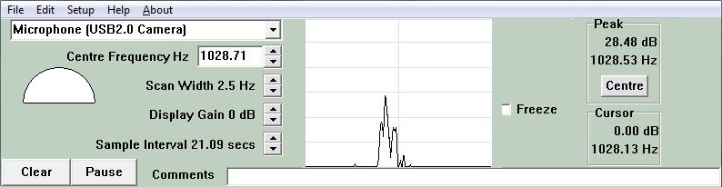
Take a look at the next picture, which is a screen-shot of the SBSpectrum software, busily receiving an 80 metre signal.
SBSpectrum operating on 80 m.
(Click on image for full-size picture)SBSpectrum runs at a sound device sample rate set in the Setup menu. The default value (8000 Hz) should be quite suitable for all modern sound devices. If you know what you are doing, you can correct the actual sample rate here if the computer sound clock is slightly off. There is rarely a need to do this, but if for example a known 1000 Hz tone is displayed at 1012.5 Hz, change the 'Actual sample rate' to 8000 x 1.1025 = 8100 Hz. The setting will be saved for next time. The sample rate chosen affects the available choice of sample intervals. With 8000 Hz, you have choices in binary steps up and down from 1.024 seconds. For most HF applications, the sample rate will be very low, typically every 20 seconds or slower. (Slower than watching grass grow!) Everything else about SBSpectrum happens in real time - it's only the spectrogram that is so slow.
You should select the sound source from the drop-down box top left. When connected to a sound source, and running, you should see the incoming audio level on the semi-circular meter, top left. Adjust the level until the meter reads about midway. The meter will turn red if the sound input overloads.
As the signal is received, the Dopplergram trace will build up very slowly from right to left. The centre of the trace represents the audio frequency set in the 'Centre Frequency Hz' box, and the top to bottom frequency span will be set by the 'Scan Width' control. The Dopplergram trace builds up at the rate of one strip per sample interval. The optimum interval is set automatically, but you can change it using the 'Sample Interval' control. Detaild instructions for tuning in and recording a signal are given below.
The display in the upper half of the program window is a spectrum analyser display, showing signal levels across the selected frequency span. Stronger peaks here will record as black traces on the Dopplergram, while weak ones will be weaker shades of grey. The spectrogram range is 60dB, and is marked with 10dB increments. Signal products which don't reach the lowest 10dB mark probably won't be seen on the spectrogram. The centre frequency is also marked by a vertical line.
The frequency and signal level can be read off from any point of the spectrum analyser or dopplergram screen, by simply pointing to it with the mouse cursor. The centre frequency, scan width, display gain, and sample interval can all be adjusted with the on-screen controls at any time, but they do not affect parts of the spectrogram trace already recorded.
If you click on the spectrogram or spectrum analyser display, the frequency you click on becomes the new Centre Frequency for the dopplergram and spectrum, so take care where you click.
File
Look at the detailed screen-shot below. The menu item 'File' allows you to save either the spectrum or the dopplergram, save the spectrogram automatically or quit the program. When you first invoke 'Autosave', it will ask you to specify a file name and folder. After that, every time the screen is full, it will save a file with that name and location, with a numbered suffix to the file name. The rate at which files are saved depends of course on the 'Sample Interval'. The autosave function is turned off by invoking the option again.Edit
The 'Edit' menu item can post the spectrum or dopplergram to the clipboard for use in other applications.Setup
The 'Setup' menu provides access to the sample rate settings, as previously discussed.Help
The 'Help' menu item calls up the file SBspec.hlp, which modern Windows computers cannot read. You should either use the winhelp32.exe application (provided in the zip file) to open the file, or use this guide instead. The SBspec.hlp file is also rather out of date.
SBSpectrum controlsAt the bottom of the controls area is a text box, in which you can type comments which will be saved along the bottom of the spectrogram next time it is saved. You can see that this has been done in the examples shown above. If no message is entered, the saved spectrograms will be annotated only with date, time of saving, the centre frequency and the width or span.
The SBSpectrum time span is completely controlled by the 'Sample Interval' control, which sets how many seconds there are between samples. The 'Sample Interval' can be set manually, but if the ratio of 'Sample Interval' to bandwidth is wrong, the picture will be very smeared, either in time or frequency.What you should do is change the 'Scan Width' manually, and let that set the 'Sample Interval' automatically. So if you want to go slower, zoom in on the signal:
As you take the 'Scan Width' narrower and narrower, not only does the spectrogram slow down, but the response of the spectrum analyser display also slows down. You must be patient when making these changes, and allow several seconds between each step. Watch the carrier build up after each adjustment, before making another.
- Tune in a carrier signal so it gives a ~1000 Hz tone (or whatever you prefer).
- Set the 'Centre Frequency' to 1000 Hz (or whatever you prefer). You should see the carrier on the spectrogram and spectrum analyser.
- Click on the carrier in the spectrogram or spectrum analyser, as that will exactly centre the carrier.
- Zoom in on the carrier by stepping down the 'Scan Width' control to narrower widths. You will note that as you do, the spectrogram will automatically run slower. But the carrier may shift on the spectrogram and spectrum analyser if not exactly centred.
- Every second step or so of the 'Scan Width' control, re-click on the carrier in the spectrum analyser, to keep it centred. Keep reducing the 'Scan Width' until you reach 5 Hz 'Scan Width', or even 2.5 Hz 'Scan Width'. Then wait... and wait... while the Dopplergram is slowly painted.
F-layer Doppler effects are typically up to 1ppm, so at 5 MHz a Scan Width of 5 Hz is appropriate to start with. At 10 MHz, 10 Hz Scan Width may be more appropriate.
One useful feature of SBSpectrum is that you can run multiple instances of the program on the same signal, so therefore you can study the signal at different scan widths and speeds. You can also run multiple instances on different signals (from different sound inputs) at the same time.
Receivers
The main requirement of a good receiver for Doppler measurement is stability. Single-reference synthesised receivers are generally more stable than conventional multi-crystal synthesized Amateur radios. An oven-controlled or external reference receiver is best. Look for ex-military receivers, higher-spec marine transceivers, and modern single reference Amateur transceivers with a 'high stability' option. As an inexpensive alternative, some of the Software Defined (SDR) radios, especially those with TCXO references (such as the RTL-SDR.COM V3 or SDRPlay RSP2), will do a reasonable job once warmed up, if the shack environment is maintained at a steady temperature.It is also helpful if the receiver has AGC switched off or disabled. The reason for this is that as the signal fades up and down, the action of the AGC will in effect modulate the signal, causing artificial sidebands to appear, especially when there are two strong paths being received that are just fractions of 1 Hz apart.
It will take plenty of practice to find suitable signals to monitor and to get good results. When using an SDR, you will need to use some extra sound function (such as StereoMix or Virtual Audio Cable) to transfer the receiver sound to SBSpectrum. Remember to select this as the sound source.
If the only available receiver has less than perfect stability, warm it up on the correct settings for several hours before making recordings, and keep the shack temperature as constant as possible. Some older radios drift anew after you change bands. Don't even think of using a VFO-controlled radio!.
Transmitters
Very often you can utilise existing radio transmissions on frequencies and in locations near the path you wish to study. The advantage here is that they are often very high powered, such as short wave AM broadcast stations or idle digital transmissions. The trouble is they often go off the air, change frequency (or in the case of digital transmissions) suddenly start sending traffic! You can use an Amateur transceiver to send a continuous carrier, but they are not designed for long term key-down use, so they may overheat, and can drift.The obvious answer is to build your own. The author has a small transmitter for 80 metres which is built into a pill bottle, and can be mailed to any station willing to run a test. It is 12V operated, uses a TCXO to achieve one part in 106 stability, and puts out nearly 1W. Here is the schematic of the transmitter:
QRP Transmitter for Dopplergram measurements on 80m
(Click on image for full-size drawing)The little transmitter is inexpensive to build and easy to get going. The TCXO reference is a 2ppm unit from an old cellular phone. The output is about 500mW, quite sufficient for good Dopplergrams, and the transmitter is efficient, drawing only 100mA from a 12V supply. See the Technical Description for more information.
Practicing
By far the best signals to practice receiving with SBSpectrum are standard frequency stations such as WWV, WWVH, JJY, CHU, BPM etc. But take care - some frequencies (especially 10.0 MHz) have transmissions from multiple stations within range at the same time, which will greatly confuse the results. Shortwave broadcast stations are generally strong, and use the same frequencies each day, but may only be on that frequency for an hour or so, and may not be there at a time of day you wish to study.
You can download the latest SBSpectrum version from the Yahoo Dopplergram Group, but you need to be a member. Look in the 'Files' section. The group is worth joining, as there are other resources and also members willing to provide guidance, and also to help interpret what you see.A recent copy of the SBSpectrum executable is also available here.
Copyright � Murray Greenman 1997-2017. All rights reserved. Contact the author before using any of this material.