Frequency or Amplitude Distortion

This distortion is the result of non-constant gain or loss in the signal transfer device over the band of frequencies being used. Measurement of this distortion is more commonly known as frequency response, We might not always classify variable gain or loss as a distortion as we often shape the frequency response for a special purpose, such as in an equaliser or a filter.

Figure 1 illustrates two conventional methods of measuring frequency response. In 1(a), the test equipment used consists of a variable frequency oscillator, a calibrated variable attenuator and a level meter. Measurements are taken at sufficient spot frequencies to construct a response curve. At each spot frequency, the attenuator is adjusted until the meter reads the same for both positions of the switch shown. The Gains of the amplifier is then equal to the calibration value on the attenuator. In this arrangement, the output resistance of the oscillator must match the input resistance of the attenuator and the output resistance of the attenuator must match the input resistance of the amplifier.

Figure 1a Methods of Measuring Frequency Response from Selected Spot Frequencies

In Figure 1 (b), the voltage calibration of a cathode ray oscilloscope (CRO) is utilised to measure input and output signal voltages. At each spot frequency, the voltage gain is calculated from the ratio of output to input voltage and converted to decibel form for plotting the response curve.

Figure 1b - Another method

Figure 2 illustrates a method of plotting frequency response on a modern spectrum analyser. A sweep generator drives a variable frequency oscillator and a variable bandpass filter which has its centre frequency synchronised to the frequency of the oscillator. The frequency is swept over the band required for the test. The oscillator is fed through the device under test and then through the filter to display output level on the Y axis of a cathode ray tube.The X axis is controlled by the sweep source so that a display of output level versus fre-quency is obtained. Modern analysers provide a computer bus across which a programmable plotter can be connected. Using this equipment, a permanent record can be automatically obtained.

Figure 2 - Frequency Response Measurement using a Swept Sine Signal and Spectrum Plot

Another method, shown in Figure 3, is to feed white noise to the input of the device under test. The white noise has a uniform spectrum and hence the noise at the device output has a spectrum which images the response of the device. The output is plotted by a spectrum analyser or a dynamic signal (to be discussed later).

Figure 3 - Frequency Response Measurement using a White Noise Source and Spectrum Plot

Sqare Wave Testing

One method of assessing frequency response (and sometimes other characteristics) is to feed a square wave to the input of the device under test and examine its output on a CRO. Since the square wave is made up of a fundamental frequency and all odd harmonics, theoretically to infinity, and deficiency within the frequency spectrum, from the fundamental upwards, shows a change in the waveform. The test is subjective rather than precise but gives a good indication of the response.

For typical waveforms, including what were figures 4 to 6 (previously in this original article), now refer to Waveform and Spectrum Analysis, ref 9.

Harmonic Distortion

Harmonic distortion in any signal transmission device results from non-linearity in the device transfer characteristic. Additional frequency components, harmonically related to frequencies fed into the input, appear at the output in addition to the reproduction of the original input components.

Measurement of harmonic distortion can be carried out by feeding a sine wave into the input of the device and separating the sine wave from its harmonics at the output. Distortion is measured as the ratio of harmonic level to the level of the fundamental frequency. This is usually expressed as a percentage but sometimes also expressed as a decibel.

Sine Wave Testing

Subjective testing for harmonic distortion can be carried out by feeding a good sine wave signal into the device under test and examining the device output on a CRO. Quite low values of distortion can be detected in this way.

Some idea of the order of the harmonic can often be determined from the shape of the waveform. For typical waveforms, including what were figures 7 to 10 (previously in this original article), now refer to Waveform and Spectrum Analysis, ref 9.

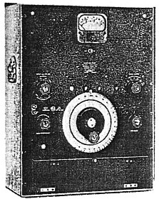
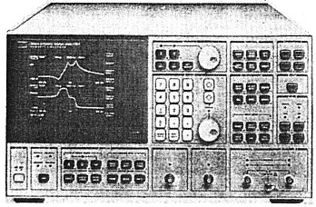
Distortion Meters

One type of distortion meter, of early vintage, is illustrated in Figure 11. The input of the device under test is fed with a sine wave source and the device output fed to a vacuum tube voltmeter (VTVM) to record a reference level. The VTVM is then connected via a bridged-T rejection filter which is adjusted to balance out the fundamental frequency. The VTVM now records the level of harmonic components and the ratio of this reading to the first reading, expressed as a percentage, is the percent harmonic distortion. To be precise, the meter actually reads distortion plus noise and noise should be taken into account if the noise level is approaching the level of harmonic component. Figure 12 illustrates the sharpness of the rejection filter and its ability to allow resolution of distortion components nearly 100 dB down. Because of the tunable filter, the instrument can measure distortion using a wide range of fundamental frequencies. Another early type of distortion meter used a fixed oscillator source of 400 Hz and a fixed high pass filter to separate the harmonic components from the 400 Hz fundamental. It had one advantage in rejecting 50 and 100 Hz hum noise components which could be a nuisance if present when using the previous instrument described.

Figure 11 - Principle of Harmonic Distortion Meter, showing Bridged T Rejection Filter composed of L2, C1, C2, & R

Figure 12 - Rejection Characteristic of Variable Tuned Filter in Harmonic Distortion Meter

Whilst measurement of total harmonic distortion satisifies a general performance assessment, there is also a need to examine the individual levels of the various harmonic components. An early type of instrument used to separate these components was called a wave analyser. Figures 13 and 14 show a wave analyser of the heterodyne type. The unit operates much like a superheterodyne receiver using a variable frequency oscillator which is heterodyned with the fundamental, or the selected harmonic, to obtain a difference frequency of 50 kHz. The difference frequency is fed through a 50 kHz narrow band crystal filter to reject all other heterodyned components and then coupled to a VTVM for measurement of amplitude. The fundamental and harmonics are selected in turn by adjusting the oscillator frequency so that a composite table of the waveform components can be recorded.

Figure 13 General Radio Heterodyne Wave Analyser

Figure 14 Basic Circuit of the Heterodyne Wave Analyser

Total harmonic distortion (Dt) can be calculated from the individual harmonic component levels H2, H3, H4, H5 etc, as follows:

D_t = √ (H2² + H3³ + H4⁴ + H5² +..... etc)

Distortion percent = 100.D_t/V_f , where V_f = level of fundamental

These early type of of distortion meters and the wave analyser described were made essentially for the audio frequency spectrum but there is no reason why the principles involved could not be applied at higher frequencies.

Another method of resolving the individual levels of the fundamental frequency and its harmonics is to display them on a spectrum analyser. Figure 15 shows a modern programmable version of the spectrum analyser made by Hewlett Packard. A typical plot, made on this versatile machine and displaying the various component levels, is shown in Figure 16. Other examples of how this type of machine can display waveform components and measure frequency response, can be seen in the article Waveform and Spectrum Analysis, ref 9.

Figure 15 - A Modern Spectrum Analyser

Figure 16 Fundamental & Harmonics displayed on the Spectrum Analyser

A further machine, used to display a composite spectrum, is the Dynamic Signal Analyser, shown in Figure 17. Whilst it can plot a display similar to the spectrum analyser, it functions on a completely different principle. A complex waveform can be resolved into its individual frequency components by a mathematical process called Fourier Analysis. The machine makes use of an internal computing system to achieve this process using an algorithm called Fast Fourier Transform. The machine can carry out a multitude of complex signal processing functions far beyond the scope of this article. Figure 18 shows a spectrum plot, made by the machine, which was set up to measure harmonic distortion. Observe how the harmonics have been separated form the noise components and each flagged on the display by an arrow. The machine has also worked out the total harmonic distortion and printed out its value at the top of the display (THD = -46dB).

Figure 17 - Dynamic Signal Analyser

Figure 18 Dynamic Signal Analyser Measurement of Harmonic Distortion

Intermodulaton Distortion

If any form of non-linearity exists in a signal processing device, intermodulation products are generated when two or more individual frequency components are fed through the device. Two individual frequencies generate two additional components equal to their sum and difference frequencies plus, to a lesser extent, more complex products involving harmonics of the two frequencies.

Intermodulation distortion is measured by feeding two different frequency sine waves to the device input and separating out the intermodulation components from the primary frequencies at the output. The relative level of intermodulation components to primary frequencies is a measure of the degree of intermodulation.

(a) (b)

Figure 19 Measurement of Intermodulation Distortion

A method of measurement is illustrated in Figure 19(a). Two sine wave signals at a frequency within the operating spectrum are fed to the input of the device under test. One signal is a high frequency (fo) and the other is a low frequency (fm). The output of the device is coupled to a calibrated CRO via a high pass filter which rejects the lowerfrequency (fm). If intermodulation occurs, the CRO displays a typical amplitude modulated waveform in which fm modulates carrier fo. Referring to Figure 19(b), percentage intermodulation equals the ratio of modulation amplitude (Em) to carrier amplitude (Ec), multiplied by 100. This is scaled off from the CRO display, as follows:

Percent intermodulation = 100.Em/Ec, [or from the diagram, % Intermod. = 100.(a - b)/ 2(a + b)]

To make the intermodulation easier to resolve, it has been past practice to feed signal fm into the device at four times the level of fo. In audio work, standard frequencies used have been fm = 60 Hz and fo = 3000 Hz.

Another method of measuring the inter-modulation distortion is to examine, on a spectrum analyser, the relative levels of either sideband component, (fo + fm) or (fo - fm), relative to fo. for one pair of side frequencies, the distortion is calculated as follows:

Percent intermodulation = 200.Vh/Vfo, or

Percent intermodulation = 200.Vi/Vfo

where Vh and Vi = sideband component levels
and Vfo = level of fo.

For further detail on intermodulation components and how intermodulation distortion is measured, refer to Intermodulation Performance and Measurement - Lloyd Butler VK5BR, ref 8.

Measurement of Phase Shift

Before discussing phase distortion, we will introduce the subject of phase and the means of measuring phase delay of a sine wave through a signal processing device. One method of measurement is to use the CRO to obtain what are called Lissajous figures. These are obtained by bridging the input of the device across the X plates input and the output of the device across the Y plates input. This method of connection was also previously discussed under the heading of sine wave testing. Typical Lissajous figures are shown in Figure 20. The phase angle is derived from sine θ which in turn is equal to the ratio of the Y intercept to the Y maximum (as explained by the diagram).

Figure 20: Lissajous Figures for Measuring Phase Difference between Two Voltages at the Same Frequency

There are various methods used to directly measure phase. The digital phase meter (Figure 21) is one such example. In this instrument, the two sine wave signals to be compared are first amplified considerably and then clipped to form square waves. The square waves are fed to a three nand gate logic circuit, the output of which is connected to a milliam meter circuit calibrated to read full scale, corresponding to 180 degrees phase shift, when a continuous one is at the logic output. For zero phase shift, the logic output is a continuous zero and the meter reads zero degrees. Tounderstand the logic, carefully examine the waveform timing diagram, Figure 22. For phase differences between 0 and 180 degrees, the average current through the meter is directly proportional to the phase difference and hence the scale of the meter is linear.

Fig 21 Digital Phase Meter

Figure 22 Digital Waveforms for Different Values of Phase between A and B

Phase Distortion

Transmission circuits and networks with reactive elements almost always introduce different phase delays for different frequencies. There is no problem if there is a linear phase characteristic, ie phase shift is directly proportional to frequency. The ratio of change in phase to change in frequency is given the name of Group Delay (Tg) which is expressed as follows:

Tg = A0/360Af

where AO = phase change in degrees
and Af = frequency change in Hertz

Variation in group delay over the signal passband is what causes signal distortion and this variation defines the phase distortion. Variation of group delay is not normally a problem in audio circuits but causes degradation of picture quality in video circuits and degradation of demodulated audio quality when present in frequency modulated (FM) signal circuits.

Figure 23 illustrates a response measurement taken on a bandpass filter using a series of amplifier stages with overcoupied double tuned transformers. The gain response looks good but observe the variation in group delay of 35 microseconds over the passband. Actually, this response is quite good and used in a narrow band FM system, produced distortion figures better than 60 dB down in the demodulated audio. This performance could not be achieved with good quality ladder ceramic filters of similar bandwidth. Such filters are notorious for their high ripple response and large variation in group delay over the passband.

Figure 23 Bandpass Filter - Gain Response & Group Delay

Group delay as a function of frequency can be plotted on automated instruments such as the HP 4192A impedance analyser. Group delay can also be measured on the HP Dynamic Signal Analyser but this instrument is limited to frequencies up to 100 kHz. Using more basic test equipment, phase shift can be measured at spot frequencies and a curve plotted of phase versus frequency. Ths slope of the curve (which is actually group delay) is scaled off around sections of the curve and a new curve, of group delay versus frequency, is then plotted.

Sine Squared Pules

We have discussed square wave as a broadband test signal which has frequency components theoretically extending to infinity. For any signal transmission system which has a controlled bandwidth, such as a video circuit, it is more meaningful to use a band limited test signal, If a sine wave half cycle is squared, it forms the pulse shape shown in Figure 24 this pulse is known as a sine Squared Pulse or sometimes a Raised Cosine Pulse. If a train of such pulses have a half amplitude duration (HAD) equal to t and a pulse repetition frequency equal to fr, then a band of component frequencies is generated, commencing at a frequency fr and extending in multiples of fr, with a band limited spectrum as shown in Figure 26. Amplitude of the spectrum falls to half (6 dB) at a frequency equal to 1/(2t) and falls to a null at a frequency equal to 1/ t. For a television video signal of 5 MHz bandwidth, values of t = 0.1 microsecond and t = 0.2 microsecond are used with fr equal to line time base frequency.



A method of generating a sine squared pulse is to feed a wide band squared pulse through a Thomson filter (Figure 25) which is specially designed to shape the signal to obtain the sine squared response.

Figure 25 Thomson Filter for Shaping Pulse

To make use of the sine squared source, the pulse train is fed to the input of the transmission system or device under test and the output examined on a CRO. Figure 27(a) shows the effect on the output when there is a loss of high frequencies accompanied by phase distortion. Figure 27(b) shows loss of high frequencies on its own. Figure 27(c) shows phase distortion on its own. By carefully calibrating the graticule of the CRO screen, limits can be defined on the amount of deviation from the original waveform than can be accepted.

Figure 27: Distortion of Sine Square Pulse

It is not intended that this article should extend into the realms of testing television video circuits although they have been referred to as an application where the sine squared pulse is used. It will be sufficient to say that a great deal of information concerning the bandwidth, low frequency response and linearity of a video signal can be obtained by studying the displayed picture of the standard television test pattern.

The Ultimate Test

We have discussed, at length, various types of distortion, the test equipment used and how distortion is measured. However, it must not be overlooked that the test equipment , whatever level of sophistication, is there to assist the evaluation of operational performance. The ultimate test is how well all the equipment performs and, in a speech communication system, how good does it sound. If the speech quality is good, then the test equipment is put away. If the speech sounds thin, or it lacks highs, or it is muffled and hard to understand, then the test equipment and the knowledge of how to use it, might be needed to find out why.

It is unlikely that the average radio amateur would have access to all of the test equipment discussed in this article. However, it should be apparent from the discussion that a great deal of information on equipment performance can be gained using a simple sine/square wave signal generator and a good CRO.

References

1. TURNER, Rufus P. Basic Electronic Test Instruments.

2. PENSKY, Sol D. Electronic Instrumentation

3. FINE, Ray S. Intermodulation Analyser For Audio Systems (Radiotronics April 1951)

4. TERMAN. Electronics and Radio Engineering

5 . Hewlett Packard Handbooks 3585A, 3562A, 4192A.

6. THOMPSON, W E. A paper - The Syntheses of a Network to have a Sine-squared Impulse Response.

7. Course of Technical Instruction -Video Test Signals - Australian Post Office.

8. Intermodulation Performance and Measurement - Lloyd Butler VK5BR

9. Waveform and Spectrum Analysis -Lloyd Butler VK5BR

Back to HomePage