![]() Ā (2.12)
Ā (2.12)
This is the
equation that must be solved to find the electric field directly in terms of
the specified current source
![]() Āor,
Āor,
i.e.,
![]()
MAXWELLÆS EQUATIONS AND BOUNDARY CONDITIONS FOR ANTENNAS:
2.2 VECTOR
AND SCALAR POTENCIALS:
|
This is the
equation that must be solved to find the electric field directly in terms of
the specified current source
i.e.,
|
|
In practice
a simpler equation to solve is obtained by introducing the vector potencial
![]() Āand scalar potencial
Āand scalar potencial
![]() .
.
![]()
![]()
![]() Ā(2.13)
Ā(2.13)
because
![]()
![]() Ā is called vector
potencial.
Ā is called vector
potencial.
(2.13) in
(2.3.a):
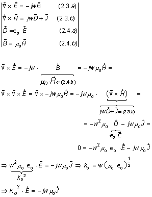
![]()
![]() (2.3.a)
(2.3.a)
![]()
![]()
![]()
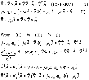
Any
function with zero curl can be expressed as the gradient of a scalar function.
![]() ĀĀ (2.14)Ā
ĀĀ (2.14)Ā
![]()
![]()
(2.3.b)
![]()
ĀĀĀĀ

Using the expansionĀĀĀĀĀ ![]()
Besides
(2.14) assumption:ĀĀĀ ![]() ĀĀ (2.14)
ĀĀ (2.14)
itÆs also
assumedĀ that Eq.(2.3.b) will hold
![]()
|
|
|
(2.13)
![]()
![]() Ā fixed.
Ā fixed.
So far only
the curl of
![]() Āis fixed by the
relation (2.13). Thus, we are still free to specify the divergence of
Āis fixed by the
relation (2.13). Thus, we are still free to specify the divergence of
![]() . In order to simplify the equation for
. In order to simplify the equation for
![]() Āwe choose:
Āwe choose:
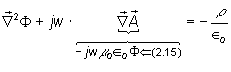
![]() Ā (2.15)
Ā (2.15)
Ā
![]() ĀĀĀĀĀ lorentz condition
ĀĀĀĀĀ lorentz condition
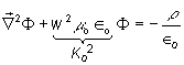
Our
equation for
![]() Ānow becomes the
inhomogeneous Helmholtz equation:
Ānow becomes the
inhomogeneous Helmholtz equation:
![]() Ā (2.16)
Ā (2.16)
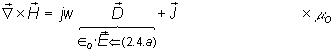
Using
(2.14) and (2.15) in Eq. (2.3.c)
(2.3.c)
![]() ĀĀ(GaussÆ Law)
ĀĀ(GaussÆ Law)
![]()
![]()
![]()
![]()
![]() Ā
Ā
![]()
However, the change is not an independent
source term for time-vary ing fields, since itÆs is related to the current by
the continuity equation (2.3.e).
(2.3.e)
![]() Ā, and it is not
necessary to solve for the scalar potential
Ā, and it is not
necessary to solve for the scalar potential
![]() .
.
Using (2.15) (Lorentz condition) in (2.14)
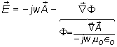
![]()
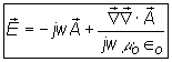 Ā(2.18)
R.E.COLLIN-ANTENNAS-p.19
The simplification obtained by
introducing the vector potencial
![]() Āmay be appreciated by
considering the case of a z-directed current
source
Āmay be appreciated by
considering the case of a z-directed current
source
![]() Āin which case
Āin which case
![]() Āand
Āand
![]() Āis a solution of the
scalar equationĀ
Āis a solution of the
scalar equationĀ
![]()
The equation satisfied by the electric field is a vector equation even when the current has only a single component.