
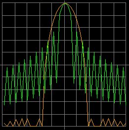
The orange trace is the spectrum display of the old version of the program.
The green line is the spectrum display of the new version of the program.
IMPROVED AUDIO SPECTRUM ANALYZER
WITH THE SOUNDCARD
(2012)
KLIK HIER VOOR DE NEDERLANDSE VERSIE
The orange trace is the spectrum display of the old version of the program.
The green line is the spectrum display of the new version of the program.

To see the improvements better, the frequency scale has been reduced here.
The orange line is the display of a signal by the old version.
The green line is the display of the new improved version.
Zero padding
As you can see, the orange line of the old version does not display the maximum. This is due to the fact that the frequency of the signal lies exactly between two FFT points. This is the so called "Scalloping Loss" and can even be 3 dB. But the green line does display the correct level. This has been solved by using Zero padding. The original FFT audio sample array of 1024 points is doubled to 2048 or even quadrupled to 4096 by adding all zeroes. During the FFT caculation, extra dots will be inserted between the original two and the maximum will be displayed much more accurate. Only 1x Zero padding or doubling the FFT sample array by adding 1024 zeroes is already sufficient for our applications.
FFT window
But you can see another improvement. At the orange line of the old version, the signal does have very high side bands. These are made in the FFT calculation and that can be solved by using a FFT window. At the green line of the new version, a FFT window has been used and the side bands are very weak. Even more than 60 dB weaker that the orange line of the old version! Unfortunately, that suppression is at the expense of the selectivity. But you can increase the selectivity again by doubling the FFT sample array (select 2048 instead of 1024).
In the old program, no FFT window has been used.
All audio samples go without attenuation to the FFT calculation.

A FFT window is a very simple operation. The audio samples of
the FFT array are attenuated in accordance with a certain curve.
 |
 |
|
A Cosine window does have already quite a good side band suppression and the selectivity is excellent. A good compromise between a good dynamic range and a good selectivity. |
A Flattop window is a very special filter. It has a flat top. Due to the flat top, it is very usable for accurate level measurements but it has a larger bandwidth. |
A Cosine window is a good compromise between a good selectivity and a good dynamic range, very good usable for a QRSS beacon reception program. A special filter is the Flat top filter. It has a flat top. That is why it is very usable for accurate level measurements. The peak of the signal does not have to be exactly on the peak of the FFT filter. For sweeping an audio filter, this is the best window.
The menu buttons
Here the explanation of some of the menu buttons. The others do not need an explanation.
Normal mode, Max hold, Average
|
In Normal mode the trace is continuously refreshed. In Max hold, the maximum value is remembered. Is the new value higher, then that point of the trace is refreshed. In Average mode, the trace values are averaged. In that way, you can make a curve of the audio characteristics of a receiver when receiving noise. Then use the Flat top window. |
FFT window
|
To select an FFT window. As explained before, it is better not to select a "Rectangle window" or no window. This window does have a bad dynamic range due to the high side band noise that is generated with such a window in the FFT calculation. A Flat top window gives the highest accuracy but also a large bandwidth, so less selectivity. When you have selected "None + DEMO" while pressing the Start button, the DEMO mode will be activated. Then you can simulate two signals and noise to see the effect of various windows. |
Rate
| To set the sample frequency of the soundcard. The higher the sample frequency, the higher the frequency range will be. The sample frequency of the soundcard is often a standard value like 44100, 48000, 96000 en 192000 Hz. But you will notice that you can also program all kind of other values for the sample frequency. How is that possible? In Windows is a routine implemented that converts the sample frequency of the soundcard to your desired sample frequency. By means of interpolation, the values of the samples are calculated from the sample values from the soundcard. At "recording devices", "advanced", you will find the setting "shared modus" and there you can set the real sample rate of the hardware. |
Samples
| To change the number of samples for the FFT calculation. This figure has to be a power of 2. Many samples does give a high resolution but a slow update time of the trace. Less samples gives a low resolution, but a faster update time of the trace. |
T=20ms
| Quite often, the first 20ms of the audio buffer was disturbed. With this scrollbar, you can set the time of that first part of the audio buffer. That part will not be used then. For my PC, 20ms was sufficient. But perhaps that this time has to be increased for other PC's. |
SOFTWARE
Download the ZIP file, unzip it in the desired directory and click the EXE file. You do not need Administrator Rights to install something, registers are not changed. There is also a ZIP file with de source code of the complete project.
Probe for the spectrum analyzer
You can make a simple probe with a 1M ohm impedance by yourself. For small signals, you can decrease the value of R1 to 10k or 1k. You can increase R2 or even remove it. The function of the diodes is to avoid damage to the input of the soundcard by limiting strong signals.

Probe for the soundcard. You can decrease the value of R1 for small signals
to 10k or 1k. You can increase R2 or even remove it.
Something about the conversion from VB6 to VB8.NET
The conversion did go automatically, except a few very essential things. Recording audio did not work anymore. That could be solved. In VB8 you cannot use "Any" and "Object" anymore. But it took two weeks before I did understand a little how that audio part did work. A problem wat that it was not possible to find some good examples on the Internet. In Python, that was much easier. After one evening it was already completely clear to me how to record and play audio whith Python.
And it was not possible anymore to draw lines in the Picture Box. That had totally been modified. You have to create a Graphic Object now. But Microsoft had a very good reason for that, the graphic possibilities are really expanded. Was it only possible to draw lines in a Picture Box, now you can draw lines everywhere, a huge improvement!
And then the screen did flicker. Much could be found on the internet about it, except a solution. The solution was found on the MSDN network of Microsoft. At first, a Graphic Buffer has to be made. Everything is drawn in this buffer and then at once copied to the Picture Box. This procedure is known as "Manually Rendering Buffered Graphics". And then the use of the PC memory did increase to even 133 Mb! As when you do use such an object, you have to do a dispose("graphic buffer name").
Something about "Marshal attributes" was in the log about the conversion. It had something to do with memory usage. All old functions from the "kernell32.lib" have been replaced by these much simpler Marshal functions and attributes.
It took some time, but Visual Basic has a great Integrated Developement Environment (IDE) and has very many possibilities and is even free for you own use. But it is quite complex. Python is much simpler and mostly sufficient for our applications. However, I will continue to play with Visual Basic NET!