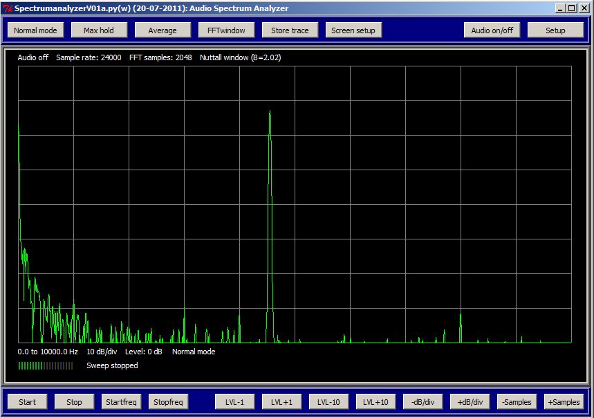
The audio spectrum analyzer program.
AUDIO SPECTRUM ANALYZER WITH SOUNDCARD AND
SOFTWARE WRITTEN IN PYTHON
(2011)
KLIK HIER VOOR DE NEDERLANDSE VERSIE
The audio spectrum analyzer program.
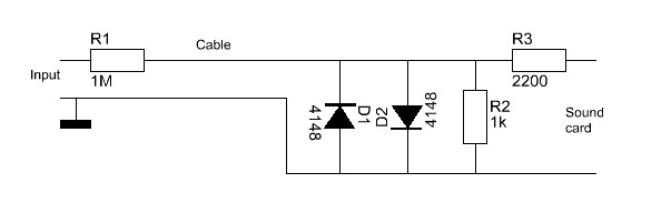
Probe for the soundcard. You can decrease the value of R1 for small signals
to 10k or 1k. You can increase R2 or even remove it.
What does an FFT window?
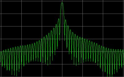
In my old spectrum analyzer program in Visual Basic, no FFT window was used (no FFT window is also called Rectangular window). Here you can choose a number of FFT windows. But what is an FFT window and what is it doing? The principle is very simple. We do read a number of samples from the soundcard and put them in a row. It has to be a power of 2 for the FFT calculation, for example 2048. Without window, all samples do have a maximum contribution to the FFT calculation. You should expect to have the optimal result, but that is not the case.
An FFT window does attenuate the samples at the beginning of the sample row and at the end. More to the center, the attenuation becomes lesser. The cental sample is not attenuated at all. But from the center to the end of the row, the attenuation increases again. So the samples at the begin and at the end of a row do hardly contribute to the FFT calculation! Why would we use a great part of the samples only partly or even not at all? And there are even FFT windows of which some samples do counteract with the other samples! The reason why we do need an FFT window can be seen here below on the various pictures of various FFT windows. No FFT window (also called Rectangular window), does generate much side bands in the spectrum of the FFT calculation. That is very well visible on the first picture. Weak signals close to the main signal are invisible. So the dynamic range is low. But by using an FFT window, side bands are much more attenuated, how much depends on the type of FFT window. But that suppression is at the expense of the selectivity. FFT windows with a very high side band suppression and therefore a very high dynamic range, do have much less selectivity. A Cosine window is a good compromise between a good selectivity and a good dynamic range, very good usable for a QRSS beacon reception program. A special filter is the Flat top filter. It has a flat top. That is why it is very usable for accurate level measurements. The peak of the signal does not have to be exactly on the peak of the FFT filter.
 |
 |
|
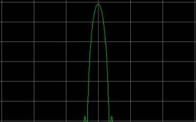
No window (also called Rectangular window) does generate very much side bands. Therefore, weak signals close to the main signal are invisible. So the dynamic range is low. |
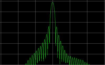
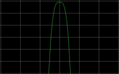
A Cosine window does have already quite a good side band suppression and the selectivity is excellent. A good compromise between a good dynamic range and a good selectivity. |
 |
 |
|
A Blackman window does have a high side band suppression and thus a large dynamic range. Weak signals close to the main signal are good visible, but due to the larger bandwidth, the selectivity is less good. |
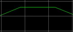
A Flattop window is a very special filter. It has a flat top. Due to the flat top, it is very usable for accurate level measurements but it has a larger bandwidth. |
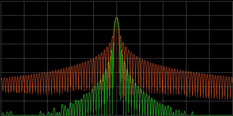
And here the Rectangular (or no) window and the simple Cosine window in one
picture, so that you can see the differences very clearly (10 dB per division).
 |
 |
| No zero padding. | Zero padding. |
Zero Padding is the solution for this problem. We fool the FFT calculation a little. For 1x Zero Padding, we double the row with FFT samples. Was the original row 2048 samples, then we add 2048 samples with the value ZERO and we do get a row with 4096 samples. What a nonsense, when we add zero's we do not add extra measurement data at all! However, something is happening in the FFT calculation with 2x as much samples. The effect can be seen in the right picture. Extra FFT frequency points are added! Coincidentally, here that extra point coincides with the frequency of the signal and the level of the signal is displayed correctly right away. But also when the frequency of the signal does not coincide with the frequency of the extra FFT point, the measuring error is already much lower. As we add samples with the value zero, the bandwidth of the FFT filter remains the same. In this program, you can choose a value between 0 and 5 for the Zero Padding. As it is a power of 2, it is a value between 1 and 32. So 0x - 31x points will be added. But the FFT calculation time will be maximal 32x longer too and the audio spectrum analyzer will slow down considerably. One extra point (a value of 1 for the Zero Padding) is already good enough to keep the Scalloping loss acceptable. And what you also can do is no Zero Padding, but take a Flat top window. The flat top is so wide, that even without Zero Padding, you will have no Scalloping loss at all. But then you will have less selectivity.
The menu buttons
Here the explanation of the menu buttons. All functions can be found under the buttons, there are no scrollbars, rotating buttons of drop down menu's.
Normal mode, Max hold, Average
|
In Normal mode the trace is continuously refreshed. In Max hold, the maximum value is remembered. Is the new value higher, then that point of the trace is refreshed. In Average mode, the trace values are averaged. In that way, you can make a curve of the audio characteristics of a receiver when receiving noise. |
FFT window
|
To select an FFT window. As explained before, it is better not to select a "Rectangle window" or no window. This window does have a bad dynamic range due to the high side band noise that is generated with such a window in the FFT calculation. A Flat top window gives the highest accuracy but also a large bandwidth, so less selectivity. |
Store trace
| No explanation required, you can store a trace with it. |
Screen setup
| To select the number of divisions on the screen. Also for selecting smaller screens. Can be handy when you want to make smaller spectrum analyzer pictures for documentation or a website. |
Audio on/off
| When you want to listen to a signal. But if there is a possibility to listen directly to the audio signal with the soundcard and the connected sound system, it is better to use that. |
Setup
|
To set the sample frequency of the soundcard. The higher the sample frequency, the higher the frequency range will be. The sample frequency of the soundcard is often a standard value like 44100, 48000, 96000 en 192000 Hz. But you will notice that you can also program all kind of other values for the sample frequency. How is that possible? In Windows is a routine implemented that converts the sample frequency of the soundcard to your desired sample frequency. By means of interpolation, the values of the samples are calculated from the sample values from the soundcard. In the setup menu, you can also input the desired Zero Padding factor (power of 2). |
Start and Stop
| Start and stop buttons for the trace. |
Startfreq and Stopfreq
| To set the start and stop frequency of the screen. |
LVL buttons
| To change the level or the sensitivity. |
dB/div
| To set the dB's per division. |
Samples
| To change the number of samples for the FFT calculation. This figure has to be a power of 2. Many samples does give a high resolution but a slow update time of the trace. Few samples gives a low resolution, but a faster update time of the trace. |
Version SpectrumAnalyzer-v01b.py
Instead of signals from the soundcard of the PC, the program can also read WAV files now. This option can be used if the frequency of WAV files have to be displayed. Before the decoding starts, the WAV files are written into memory. It looks as if nothing happens, but just wait. The variable WAVinput (line 77) has to be set to 1 instead of 0 to activate the WAV mode.
Version SpectrumAnalyzer-v01c.py
There is a possibility to store the trace as a .CSV file [frequency,dBlevel], an idea of Jack Lindsay. The screen has been enlarged and the conversion routine from dB's to screenpixels has been optimized.
Version SpectrumAnalyzer-v02a.py
The speed has been improved, mainly by replacing some routines by Numpy routines. And a time / date stamp is added to the file name when storing the trace as a .CSV file [frequency,dBlevel].
Version SpectrumAnalyzer-v04a.py
For Python version 3 and 24 bits WAV files.

PC off! Finally finished!
And then someone came with a new idea...
SOFTWARE
Before you are using this program, you have to install Python. That is very simple. But read first something about Python by clicking the following link:WHAT IS PYTHON AND HOW DO YOU INSTALL PYTHON
As the source code of Python is written in ASCII, it is very simple to modify the program to you own requirements. Think for example about the size of the screen, the colors etc.
Required Python version:
Download here the Python spectrum analyzer program by clicking the link here below: