
I hope amateur radio astronomy enthusiasts can benefit from this reading in the meanwhile though.
Michael Fletcher, 26.04.1999
-------------------------------------------------------------------------------------------------------------------------------
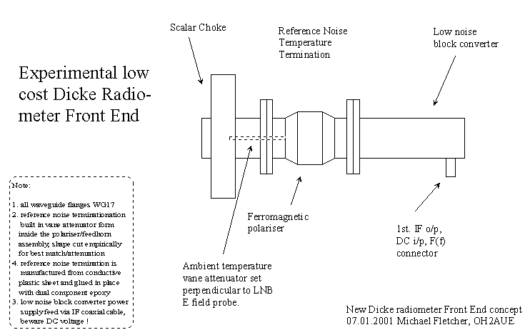
P.S. see my drawing of an experimental Low Cost Dicke Front End: >25 dB of broadband cross polar (hot/cold) isolation :-)
Michael Fletcher, 07.01.2001
-------------------------------------------------------------------------------------------------------------------------------
Michael Fletcher, OH2AUE
A Microwave Dicke Radio Telescope for the Amateur
====================================
Foreword
-----------
In this article I describe the background of a project of mine that
has been continuing for several years now. The main
objective has been to construct a very sensitive and high resolution
microwave radio telescope suitable for the average
radio hobbyist.
Preface
-------
Years ago a student colleague of mine did some very interesting experiments
with a 100 MHz receiver and a couple of Yagi
antennas configured as a phase swithching interferometer with which
he had succeeded in making some impressive noise flux
measurements from celestial sources. He was very interested in astronomy
and this is what booted this engineering student
into the wide world of radio astronomy. In his system the Yagis where
configured in the phase switching interferometer
mode and the idea was largely based on a series of articles ( 6,7,8
) in the Sky and Telescope magazine.
My friend was more interested at the time in celestial objects than
I was, but my main interest has always been weak signal
techniques in the amateur radio domain, and especially at microwave
frequencies, so our interest areas found some common
ground to re-establish the radio telescope workshop....
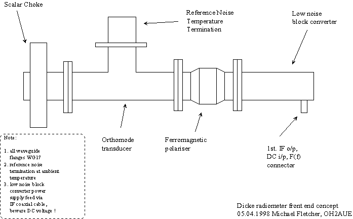
The Microwave Enthusiasts Solution
-------------------------------------
Several years ago now, mass produced Ku-band satellite TVRO ( TV Receive
Only ) equipment started to make it's way
into the market. By this time I already routinely used the sun as a
reference noise source for checking my 10 GHz ham gear in the
total power measurement mode. Mass production of these components really
dropped the price of microwave devices and
components particularly in this band as had already happened to C-band
components.
What I was really interested in was modifying the interferometer back-end
circuitry in order to use it as a so-
called Dicke switch comparison radiometer at microwave frequencies.
Note: By the Ku-band one means the 12.4 - 18 GHz range by old designation,
but this generally is ( incorrectly ) used to
describe the combined 10.7 - 14.5 GHz satellite downlink and uplink
bands. C-band would be equivalent to 4 - 8 GHz, and
this is similarly used in "TVRO lingo" to describe the combined corresponding
uplink and downlink frequencies. L-band
is also an old designation still widely in use, and it refers to the
1 - 2 GHz band, but again the TVRO industry intends the
750 - 2150 MHz IF ( intermediate frequency ) band commonly used in
satellite TVRO receivers.
Problems
----------
First of all, as I wanted to construct a continuum receiver, the detection
bandwidth was to be as large as practically
possible. Now this wasn't conveniently done with my 3 cm rigs without
more or less completely dismantling the
equipment and reassembling it in a different manner, and besides, I
needed that equipment for other purposes !
The second problem is the high temperature instability encountered
in this type of total power radio meter. If the
reception chain incorporates say 150 dB of gain distributed between
the RF stages and the post detection stages,
the gain variation in the complete chain is considerable setting a
practical limit to the maximum usable gain in the system.
Particularly if the receiver has been designed from a completely different
stand point.
First Experiments
-----------------
The first experiments with these commercial TVRO components was a simple
radio meter comprising a 28 cm offset
parabolic dish ( 37k ) with a 12 GHz front
end boasting a high 2.5 dB noise figure. I then simply added sufficient
IF
gain in the 1 GHz region so as to be able to use a diode detector for
level measurement and even a thermocouple power
meter. The gain variation problem was imminent and obvious after a
few hours plotting on an old strip recorder, but the
solar detection capability was impressive. The cold sky versus hot
ground noise difference was even greater, as the
antenna could see these noise temperatures with the full aperture,
whereas the sun represents approximately 0.5
degrees
of viewing angle. The corona will expand the radio diameter somewhat.
Just to keep things simple let it suffice to say that
noise temperature is just another way of expressing noise figure and
losses, albeit a better way though. It is easier to add
and subtract noise temperatures directly rather than going through
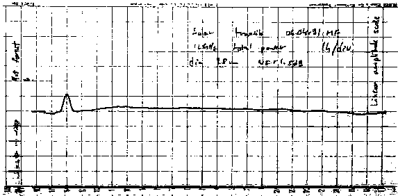
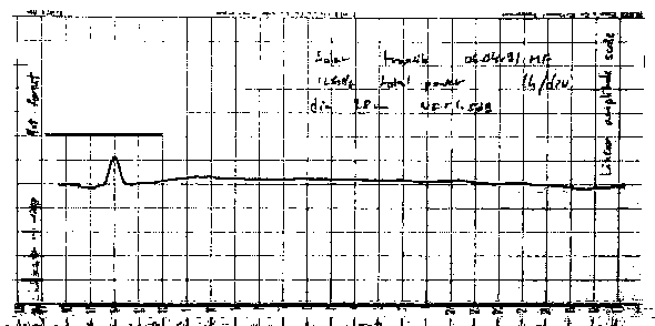
the dB conversion rigmarole. This entire subject is
discussed in total detail in reference ( 1. ). Here is a similar
plot of a solar transit with cold sky as the
background except
for a period of time when it snowed and the perforated offset dish
was totally washed with snow ( broad peak of
apparently hotter noise temperature to the right of the solar transit
).
At this stage I also put together an IF system downconverting from the
L band IF to 480 MHz using a satellite TV tuner
from which I extracted the IF and disabled the AGC/limiter. This 480
MHz IF I then fed to a regular TV tuner further
downconverting to the 33 - 39 MHz standard IF resulting in a predection
bandwidth of 6 MHz. Some satellite tuners use
an IF of 608 MHz too, but they all work similarly and are adaptable
for this type of project. This concept also allowed
me to tune the microwave reception frequency ( at the L-band IF ) enableing
reception even "between" satellites. Here
is a plot of the predetection IF taken with
my homemade spectrum analyser. The vertical scale is 10 dB/division and
the
horisontal dispersion is 10 MHz/division. The spike at the left is
the zero frequency ( DC ) reference.
These two arrangements enabled measuring of solar noise temperature
at ease. Finding the noisy ball through massive
overcast posed no problems whatsoever despite the poor sensitivity
of the arrangement.
The First Measurements
------------------------
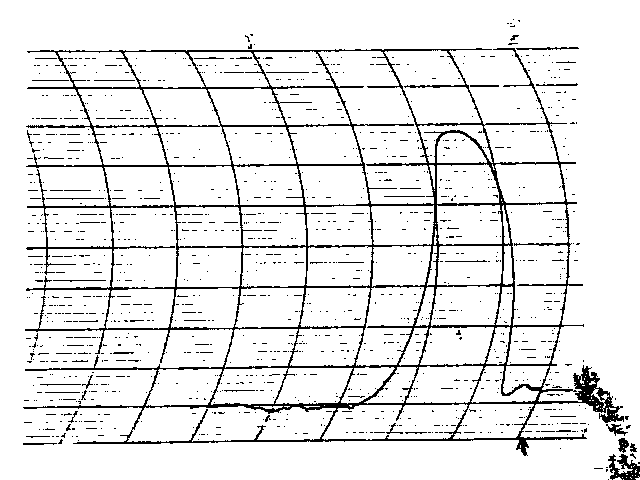
Here is an early plot using the above mentioned 12 GHz receiving
system. Note the 290 K forest noise level being
apparently higher than the approximately 10000 K sun. The amplitude
scale is linear ( the detector is operatind in the
linear range ) and the time scale is 1 hour per division.
Action Time
------------
In my first measurement I did not even use the strip recorder, I just
observed the total noise power with the thermal power
meter. This is a home brew power meter ( 61k )
giving reasonable accuracy from DC to 11 GHz and is based on an article
in the European VHF Communications Magazine. At one stage I used the
DC measurement result for driving an audio
function generator in the VCO ( Voltage Controlled Oscillator ) mode.
The loudspeaker would then emit a tone whose
pitch would vary according to noise temperature. An early version on
the Dicke radio meter ( 50k ) to be descibed
later
was actually demonstrated at a national astronomy meeting in such a
way, that the antenna pointed towards the cold sky
at a low elevation though triple glazing ( ! ) glass over a staircase.
Exhibition attendees then walking up the stairs into the
antenna beam would distinctly hear the rising tone from the VCO/generator
as the persons microwave noise temperature
was sensed by the radio meter. Needless to say, people were impressed
- and worried. Hopefully we succeeded in
boosting the interest in amateur radio astronomy.
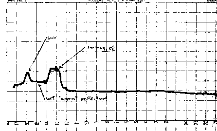
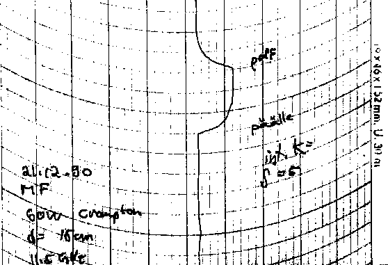
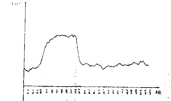
This narrower band early radio telescope equipment was quite impressive
in it's perfomance. It was quite trivial to detect
the microwave radiation of a regular 60 W incandescent lamp located
15 cm in front of the antenna feedhorn ( having an
approximate beamwidth of 120 degrees ). This is an
analogue
plot of this effect and this is a digital plot
of a similar experiment.
Anyway, the VHF Yagi system got the boot, but the back-end was preserved
for technical research and development.
Instead of switching phasing lines via PIN ( used for RF switching
) diodes, it was modified for use as a Dicke detector.
Imagening what could be done with a 1.5 m or 3.0 m dish and modern
GaAs-FET's and P-HEMT's is mind boggling.
Of course the quantity of detectable noise sources drops, but it is
quality that counts. With these type of antenna apertures,
the spatial resolution becomes reasonable per real estate, and I haven't
even started on the long baseline interferometer or
correlation spectrometer yet !
More Action
-------------
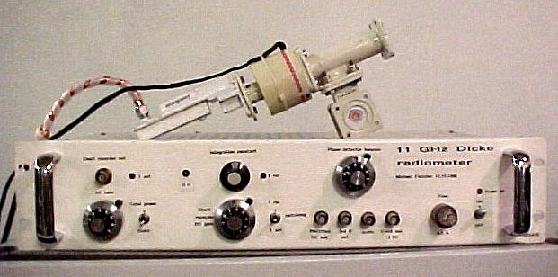
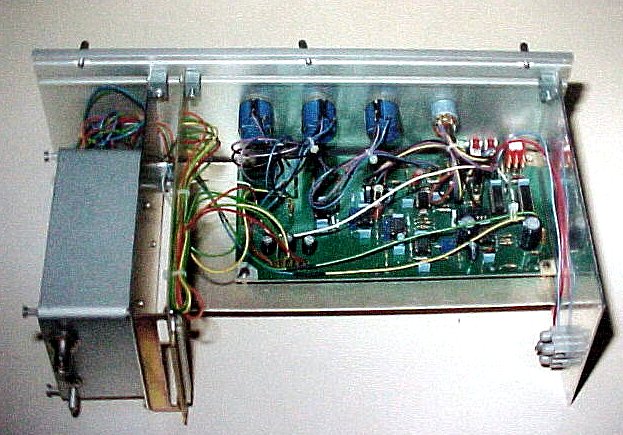
The next stage was to construct a combined total power radiometer and
so-called Dicke radiometer ( 88k ).
In the Dicke radiometer particular arrangements are made so as to eliminate
to great extent the the gain
variation over time previously described using the comparison method.
What the reference compared to is,
defines the final gain stability.
Here is a short description of the original Dicke radiometer used by
R.H. Dicke ( 1. ) himself. The basic
principle is to show the receiver ( the balanced waveguide mixer also
called the Magic-T ) alternately the
antenna noise temperature and that of the reference load. This swithching
problem Dicke solved by machining
a slot down the middle of a TE10 mode waveguide ( this can be done
without the slot interfering with the
propagating wave in any way ) into which he inserted a rotating disk
half of which was insulation material the
other half being absorptive material. As the disk rotated in the waveguide
it alternately was more or less
transparent half the time and the other half it appearded as a well
matched attenuator. Of course it is obvious
that there are imperfections in this type of modulator such as the
modulation function being sine-like, but it
served the idea Dicke had in mind. Actually there was a lot of consequent
discussion in many technical journals
and publications of the time about this matter ( 2,3,4,5 ), but hey,
the man measured lunar noise temperatures
in 1946 with valves and diodes !
The synchronous detector ( "coherent detector" ) in the receiver operates
at the same angular frequency as
the disk modulator, so it now becomes possible to use significant tuned
amplifier AC gain after the envelope
detector and before the synchronous detector. This of course also caused
some discussion, as the ideal
switching waveform would be square, which it isn't if the signal harmonics
are filtered out, but let's let it pass.
Now taking a look at the whole system, it is obvious that ( almost
) all gain variation after modulation and
before synchronous detection is the same for both the measurement source
noise power and the reference
temperature termination noise power, especially when they are in the
same ball-park. There is actually a
variation of the described system in which the reference noise power
is automatically readjusted to be the
same as the measurement source power, thus making the system inherently
gain stable.
Dicke: The resolution
----------------------
The resolution of a Dicke-type radiometer is:
In which;

It can be seen, that the last term consists of the multiplication factor
of gain variation and the of the antenna and
reference termination noise temperature difference. So, if the reference
termination noise temperature is same as
that of the antenna, the gain variation term is eliminated. On the
other hand, when measuring very low noise
temperatures, such as celestial sources ( other than the sun ), it
is advantageous if the reference noise temperature
is as low as possible.
In some radiometer solutions, where the measured noise temperature is
high, like when measuring earthly objects, one
can use an actual noise generator as the noise power reference. The
noise power difference is then zeroied with the
measurement result from the integrator. Since the last term in the
equation is now eliminated the gain variation factor is
out of the game and the integrator output of the formed closed loop
is equivalent to the measured noise temperature.
Brightness Temperature vs. Physical Temperature
--------------------------------------------------
Brightness temperature and physical temperature bear the following relationship:

A Reference Colder Yet
-------------------------
In my first experiments I simply used a high quality termination as
the cold reference, but recently I have also
experimented with the so-called cold sky reference in which the resistive
termination is replaced with a horn
antenna that is pointed towards a cold spot in the sky. During long
term measurements it would be advantageous
to point the reference horn towards the Galactic north so as to maintain
a constant noise temperature ( easy for me
to say at these latitudes... ) except for atmospheric variations and
the physical temperature of the horn. The latter
is compensated automatically as a bonus though, since it is at the
same temperature as the measurement antenna.
Another Cold Rererence
-------------------------
The most convenient method of cooling the termination would be to use
dry ice, nitrogen ( 77.3 K ) or even
helium ( 4.2 K ). Of course this would require purchaseing a Dewar
of some sorts, and these cost typically
more than the rest of the described equipment. A 10 l Dewar costs around
600 USD here in Finland, but it
does come with a five year guarantee. Boiling water is useful for a
hot reference at 373.2 K and another stable
temperature can be obtained easily from melting ice at 273.2 K.
Other means of increasing resolution could be increasing noise detection
bandwidth or integration time
constant, but both have their penalties.
What Resolution Can Be Achieved
------------------------------------
Lets look at one of my radiometers as an example. The terminations
used is at room temperature
( approx. 290 K ):

These values result in a delta-T of 7.8 mK.
This kind of resolution is very good indeed. A receiver with this resolution
will also react to very minute changes in noise temperatures seen by
the antenna. Small clouds and any type
of humidity will be readily seen on the output of the receiver and
in this way we have actually succeeded in
reaching this limit of sensitivity - the only two things that can be
further improved are increasing antenna
diameter and stabilizing the reference temperature by cooling with
a controlled system.
If the reference termination noise temperature where to be 40 K and
the receiver noise temperature to be
105 K, the resolution whould end up being 2.9 mK with a reasonable
integration time constant of 20 s.
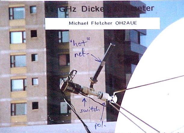
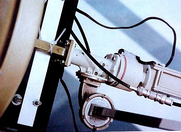
Innovative Misuse
------------------
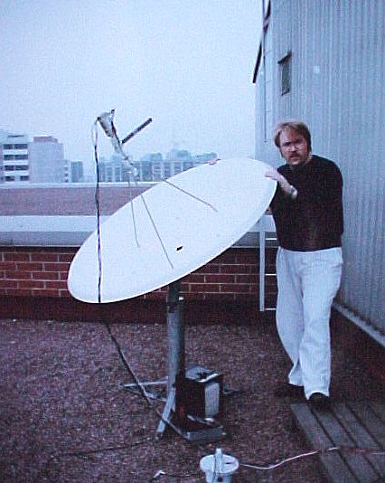
In this particular solution ( photo, 50k )
the comparison switch is made from the combination
of a so-called
OMT ( orthomode transducer, used for vertical and horizontal polarisation
separation in TVRO use ), which
is basically an E- and H-field combiner, and a electromagnetic polarizer
used originally for selection of desired
polarisation to the LNB ( Low Noise Block ) input. This is based
on a phenomenon called Faraday rotation
and utilizes the characteristics of a particular type of ferrite and
its bahaviour when subjected to a magnetic
field, which may be either permanent of generated by DC current, as
in this case. As ferotors, as these
commercial gadgets are called, are not designed for rapid swithing
( the switching rate in the Dicke receiver
should be in the order of 10's of Hz and up, as the gain fluctuations
are typically in the range of Hz and less )
we face the first problem, which is to identify a polarizer suitable
for switching purposes. Well, I have tested
many different types and most of them are usable at about
10 Hz, but those manufacured my IRTE and
Swedish Microwave ( 88k ) here in Europe
enable switching rates of 20 - 25 Hz to be used too. The practical
difficulty is the remanence magnetic field causing a time delay between
switched states and if the delay is too
long the synchronous detector will not operate in a satisfactory manner.
The ferotors are typically driven in the
current mode being of the electromagnetic variety, but a suitable accuracy
of 90 degree switching of planes is
possible with a simple 0 / 5 V switching signal. The perfectionist
of course would consctruct a dual current
supply switcher, which isn't too difficult with an LM317 for example.
A method of alleviating the remanence
field problem ( the field strength is proportional to the square of
electric current in the coil ) is to use a current
or voltage switching signal that is symmetrical about 0 mA or 0V (
e.g. +/- 2.5 V instead of 0/5 V ). The
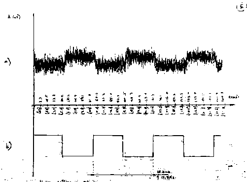
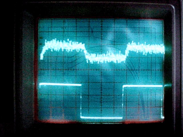
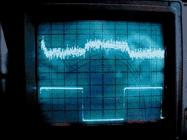
switching waveform can be readily monitored on a cheap low frequency
oscilloscope by using the swithching
signal on channel A for monitoring scope triggering and watching the
postdetection noise waveform on
channel B ( Fig. 4a, cold source, 65k )
and ( Fig 4b, hot source, 69k ).The improvement
of using a square
wave switching waveform over a sinuous waveform is approximately
10 %. Actually, while watching the
noise waveform it is possible to define the cross polarisation leakage
by using a regular flourescent lamp or
gas discharge lamp as the noise source into the antenna port. The noise
is distinctly identifiable through the
modulation caused by the mains AC voltage. In this way the polarisation
setting current or voltage can be
easily optimized without hi-tech equipment.
In my experiments I have connected the reference horn to the OMT via
a short length of surplus ship radar
X-band flexible waveguide I have built adapters for. In my prototype
version I adjusted the optimum
polarisation angle by rotating the ferotor and re-drilled new holes
in the flange for bolting down to the new
angle. The 90 degree position can then be adjusted by voltage/current.
( X-band is the commonly used old expression for the 8 - 12.4 GHz band )
What Is Detectable
--------------------
When using the mentioned figures and a 3 m dish with a 50 % illumination
efficiency, it should be
possible to achieve a sensitivity of about 5 Jansky's. It would thus
be possible to measure the
following noise sources ( Fig. 5 ):
Crab Nebula ~600 Jy
Cassiopeia A ~700 Jy
Cygnus A ~100 Jy
Orion Nebula ~500 Jy
Jupiter ~70 Jy
Mars ~14 Jy
Virgo A ~40 Jy
M31 ~60 Jy
For calibration purposes one can readily utilize the moon
at approx. 200 K and the sun at approx. 11 000
K,
both at 11 GHz. It should be realized that the solar noise temperature
varies very much indeed, especially
during periods of solar activity ( sun spots ). Even the lunar noise
temperature varies a few tens of Kelvin at this
frequency depending on lunar phase. This in it's self is an interesting
object to measure, as it is possible to draw
conclusions on the surface construction of the moon, as the radio temperature
and optical ( Infra red )
temperature have a noticable delay over phase. Note the raggedness
of the lunar plot, which is due to the
very light overcast that prevailed during this nocturnly measurement.
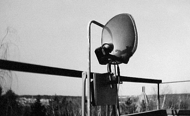
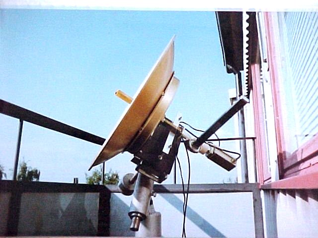
The measurements in figures 6 & 7
were made with a 1.3 m parabolic prime focus dish, with the microwave
assembly at the focus ( photo, 55k ).
The aperture blocking is of course one source of imprevement. This
dish size is also suitable for the city dweller
if you have a balcony ( 62k ) or other access
to an open spot. I have also done some experimenting with a
60 cm dish ( 52k ) on my balcony with less
blocking walls and railings and have also detected the moon
easily with a 28 cm prime focus dish and one of my Dicke receivers.
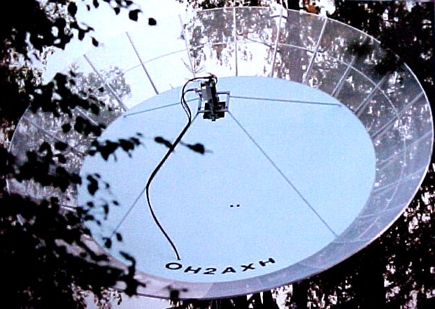
I also have access to a home-brew 6.4 m dish
( 77k ) that has been built around a 4.5 m old parabolic radar
antenna. This antenna is useful to at least 10.5 GHz and it was used
for the very first EME contacts on 10 GHz
from Finland in the summer of 1995 ( Earth-Moon-Earth ).
Other Improvements
---------------------
Several improvements have taken place over the years. One of the more
notable ones was the
implementation of a temperature compensated
envelope detector ( 85k ). This may come in many
forms, but the one I have in use now is from an article in the QST
magazine of December 1991.
It is now possible to icrease the system gain by a step further as
this temperature drift source has
now been eliminated.
Well, this improvement brought to hand the next problem, namely the
physical temperature variation
of the outside antenna and switched reference
( 67k ) system. You get the diurnal temperature
moving the chart strip recorder pen from end to end of the most sensitive
scale, so an electronic
compensation of the physical temperature comes to mind as preferred
to thermally stabilizing the
whole microwave department at the dish antenna prime focus. When using
the cold sky reference
horn, the system sensitivity is so high that sidelobe effects, aperture
blocking effects and reflection
of ground noise via the feed support struts are seen with ease. So
the rat race has commenced.
The project is seemingly never ending, and this is one of the reasons
why this project stays high
on the interest scale.
Reference Construction
------------------------
The reference can be easily made to suitable matching values with the
conductive
foam ( 5k ) used
for protection of static sensitive devices. Try to find some of the
better conducting variety, this is
easily measured with a multimeter. This should be cut to a long
( > one wavelength ) pyramidal form
with an Exacto-knife or similar and glued to the bottom of the used
waveguide section ( Fig. 9 ).
The waveguide can be made from sheet brass. Don't let anyone discourage
you about the
accuracy required for microwave devices just do it - you'll be
surprised !
The reference may also be treated more scientifically and Peltier cooling
isn't too hard a subproject
either. The isolation of the termination from the rest of the waveguide
system can be achieved by
using a sheet of PTFE between flanges and using Nylon screws. The system
should be thermally
isolated by enclosing the termination ans a reasonable length of waveguide
in a Styrox box. The
cooling fan needed by the Peltier elements has to be suitably located
so as not to blow the pumped
heat onto the other waveguide parts. As the waveguide components have
quite low losses, their noise
temperature contribution is not consirable, but it will be if we continue
to improve the system at this rate !
Other Telescope Solutions
---------------------------
I have dismantled tens of different TVRO LNB designs for various reasons
like modifying them for
amateur television ( ATV ), SSB/CW use on amateur satellites ( the
new AMSAT Phase III D satellite )
and radio astronomy projects. What I have been particularly interested
in is finding suitable methods
for modifying these LNB's for crystal control use ( phase locking,
injection locking, external LO etc. )
and modifying the frequency response to the amateur band 10.000 - 10.5000
GHz.
Most 4 GHz units are usable for the 3.4 GHz band ( those that have
it ) and also radio astronomy.
The construction varies greatly, but some types are particularly easy
to modify. If we consider two
LNB's that were phase coherent through injection locking or via a common
external local oscillator,
we can't avoid thinking of constructing a long base interferometer,
in which we have two antennas
each with their own common LO LNB, the IF's of which are processed
so as to form an interferometer.
The spatial resolution of this can be derived from the baseline length
i.e. the apparent antenna aperture
is based on the distance between antennae. So you can see that if the
sensitivity of the receiver system
is sufficient to measure the noise flux of the source we are interested
in, the angular resolution with which
we can study the object is based on the baseline length. Imagine mapping
the solar or lunar surfaces with
a backyard "VLBI" telescope ! Or if you are inclined to mathematics
processing on a PC you could
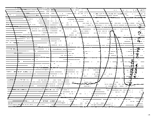
easily construct a cross correlation spectrometer ( see simulated example
in Fig. 10 ).
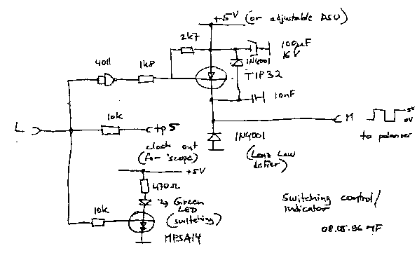
Circuit Description
-------------------
The circuit to be described is based on the design of G.W. Swenson and
K.-S. Yang. The operational
amplifiers have been changed to more stable types, the switching logic
has been modified to CMOS
technology and the detector is using the previously described temperature
compensation. Also the total
power optioin has been discarded. I wouldn't recommend this though,
I re-implemented the DC-coupling
option in my consequent back-end design.
The temperature compensated envelope detector is constructed a fairly
straightforward manner. The measuring
diode and temperature compensation diode are slightly forward biased
to optimise the dynamic range.
The sensitivity of the detecor is such, that linear response is achieved
with an input range of around
- 35 dBm to + 5 dBm. To maintain this kind of level, the detector is
preceeded by three MMIC
amplifiers. The types used in the prototype were manufactured by Avantek
( HP ), but there are
equivalent types from Mini-Circuits too. The interstage coupling capacitors
are in the tens of picofarads.
In this way the frequency response in possible to keep useful about
10 MHz to approximately 1 GHz.
A later version used 2 GHz MMIC's in order to reach a predetection
bandwidth of well over 1 GHz.
The first amplifier input circuitry incorporates an RF choke before
the DC decoupling capacitor for feeding
the necessary DC voltage required by the LNB. This DC line should be
supplied with a fuse and switch
for protection and in case the back-end might be wanted to use for
VHF or UHF detection.
A suitable signal generator for measuring the bandwidth and the frequency
response can be readily made
from a VCO unit as available from many manufacturers as a building
block. These typically come with
the frequency/tuning voltage dependancy specified reasonably well in
the respective data sheet.
This is a straighforward amplifier stage in order to reach the desired
AC signal level before entering the
synchronous detector.
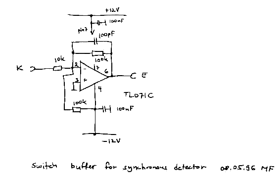
This synchronous detector is a regular design. The switching FET is
driven by an OP-amp stage. The trim-pot
on the negative input is used for gain equalisation as per the original
design.
The basic clock is based on the popular 4060 oscillator/counter and
the prototype used a manually selectable
RC time constant for experimenting with various values. The following
JK-flip flop is configured is such a way
that the switching can be stopped and the stationary noise entering
the detector is selectable between the
antenna or the reference termination. This enables various measurement
possibilities especially if the total
power measurement option is used.
In the prototype, the switching voltage is simply 0 or 5 Volts and as
previously mentioned an implementation
of a dual value current generator would be advisable. The Cal. output
is used for gain and balance calibation
as per the original design in
Sky & Telescope.
The front panel has three LED's indicating the clock circuitry status;
one green blinking LED to indicate
switching and two red LED's to indicate the stationary state of measuring
either antenna or reference noise power.
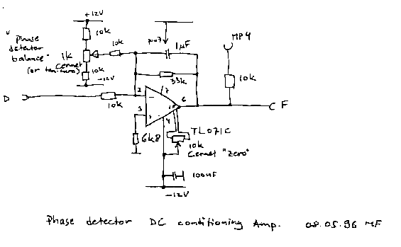
5. Phase sensitive detector balance control
The stage following the phase sensitive detector is used for offsetting
the DC base component coming from the
detector circuit. In this way the measurement result would be above
the base value of zero Volts.
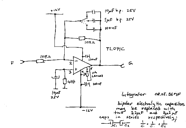
The integrator is very similar to the original design. This is a standard
OP-amp solution. Of course
a more advanced circuit would work well or better here, but the circuit
complexity isn't worth the
effort in my opinion. When changing time constants, the stabilisation
period will depend on the constant
of course. The selection switch should be of reasonable quality due
to the high impedances. The
contacts should preferrably be hermetically sealed to maintain continuous
multi-year operation,
particularly as the back-end will possibly be used sometimes in a not
so ideal environment.
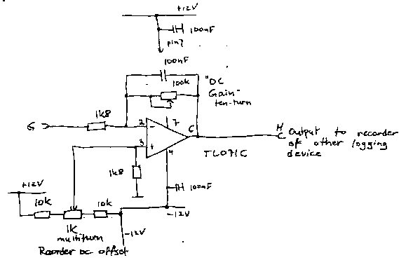
7. Strip chart recorder driver
The final amplifier is used for giving control over the strip chart
recorder output. Both gain and offset
are adjustable. The output is suitable suitable for a 1 mA full scale
deflection. I have several resistor
loaded outputs here, because I also want to feed the measurement result
to the audio VCO and a
multimeter that has an RS-232 interface to a computer.
8. Power supply
The power supply is straightforward and can use either adjustable regulators
of the LM317/LM337
variety or fixed regulators of the 7800/7900 variety. If the radiometer
is to be constructed using
TVRO satellite and TV tuners, it is necessary to implement a low current,
stabilized voltage of
about 20 - 33 V for tuning purposes depending on the tuner types used.
If switchmode power
supplies are used, special care must be taken to assure that no switching
transients are allowed to
enter the DC power lines in the radiometer.
Appendix
----------
Here is a list of interesting further reading on the subject. I very
positively recommend laying hands
on the book Radio Astronomy compiled by J.D. Kraus for the even remotely
interested amateur
radio astronomy enthusiast. The book is considered as being the bible
of radio astronomy my many.
1. Kraus, John D., Radio Astronomy, 2nd ed. Cygnus-Quasar
Books
2. Johnson-Jasik: Antenna Engineering Handbook, 2nd ed.,
chapter 31: Bailey, M.C., Coswell, W.F., Radiometer Antennas
chapter 41: Kraus, J.D., Radio Telescope Antennas
3. Anderson, M.D., Landecker, T.L., Routledge, D., Smegal, R.J.,
Trikha, P., Vaneldik, J.F, Ground Radiation Scattered
from Feed Support Struts: A Significant Source
of Noise in Paraboidal Antennas, Radio Science, vol. 26, No. 2, March-
April 1991
4. Anderson, M.D., Landecker, T.L., Routledge, D., Smegal,
R.J., Vaneldik, J.F, The Far Side Lobes and Noise
Temperature of a Small Paraboidal Antenna
used for Radio Astronomy, Radio Science, vol. 26, No. 2, March-April 1991
5. Smith, J.R., A Basic Radio Telescope, Parts 1 & 2, Wireless
World, February, March, 1978
6. Gibbins, C.J., Cherry, S.M., The Effect of Spatial Inhomogeneities
on the Elevation Angle Dependance of Atmospheric
Thermal Emission at Millimetric Wavelenghts,
Radio Science, vol. 24, January-February, 1989
7. Wagner, L.A., Measuring the Accuracy of a Parabolic Antenna,
Ham Radio Magazine, September, 1989
8. Stokke, K.N., Fro/sland, T., Change in Noise Conditions due
to Losses and Thermal Radiation, Telektronikk, Nr 2. 1989
9. Taylor, R.E. 136/400 MHz Radio-Sky Maps, Proc. IEEE, April
1973
10. Melhuish, S, Cosmic Conundrums, BBC Acorn User, March 1993
11. Jirmann, J., Radio Astronomical Experiments in the 70 cm Band,
VHF Communications, 3/1994
12. Lambert, K.M., Rudduck, R.C., Calculation and Verification of Antenna
Temperature for Earth-based Reflector
Antennas, Radio Science, vol. 27, no.
1, pages 23 - 30 January-February 1992
13. Compton, J.R., An Alignment Aid for VHF Receivers, Radio Communication,
January 1976
14. Carr, J., Noise, Signals and Amplifiers, Ham Radio Magazine, February
1988
15. Sly, T., Noise Figure Indicator, QST, January 1965
16. Hagn, H., Receiving System Parameter Measurements using Radio
Stars, VHF Communications 2/95
17. Haykin, S., Li, X.B., Detection of Signals in Chaos, Proc. IEEE,
vol. 83, No. 1, January 1995
References
-----------
This is a list of references made in the text:
1. Dicke, R.H., The Measurement of Thermal Radiation at Microwave Frequencies,
Rev. Sci. Instr., vol. 17, July 1946
2. Goldstein, S.J. Jr., A Comparison of Two Radiometer Circuits, Proc.
I.R.E., vol. 43, 1955
3. Tucker, D.G., A Comparison of Two Radiometer Circuits, Proc. I.R.E.,
vol. 45, 1957
4. Strom, L.D., The Theoretical Sensitivity of the Dicke Radiometer,
Proc. I.R.E., vol. 45, 1957
5. Galejs, J., Comparison of Subtraction-Type and Multiplier-Type Radiometers,
Proc. I.R.E., vol. 45, 1957
6. Swenson, G.W. Jr., An Amateur Radio Telescope, parts I -XI, Sky
& Telescope, May - October 1978
7. Swenson, G.W. Jr., Antennas for Amateur Radio Interferometers, Sky
& Telescope, April 1979
8. Swenson, G.W. Jr., Franke, S.J., An RF Converter for Amateur Radio
Astronomy, Sky & Telescope, November 1979
(Minor improvements 11.01.2003, Michael Fletcher, OH2AUE)