Computer Assisted Low Profile Antenna Modeling II
Computer Design of a Low Profile Horizontal Loop
Antenna for a Limited Space Backyard
by Dr. Carol F. Milazzo, KP4MD (posted 25 September 2010, updated 18 Feb 2018)
E-mail: [email protected]
SUMMARY
This article describes the application of computerized
modeling to design and analyze the performance of a low
cost, low profile horizontal loop antenna that exhibits
gain over a dipole within a limited space backyard using
household materials and low cost speaker wire zip cord as
the transmission line.
INTRODUCTION
I first experimented with
antenna modeling in 19971 when I moved
to a residential housing development where restrictive
covenants did not permit outdoor antennas. The
space available for antennas at that time was inside a
peaked roof attic. In 2006, I moved to a mobile
home park with covenants that restricted antennas
visible from the street. My first antenna at this
location was a remotely tuned base loaded 6 foot
vertical whip antenna (High
Sierra Sidekick) mounted on the roof at the rear
of the home. The aluminum siding served as its
counterpoise. Its observed performance was fair on
21 and 28 MHz, mediocre on 7 and 14 MHz with little
reception except to the north, and overall quite poor on
3.5 MHz. Seeking better performance on the lower
frequencies, I later installed a 100 foot end-fed random wire antenna of
20 gauge insulated stranded wire supported by
two 15 foot PVC poles at the south corners of the
property. That antenna performed marginally for
contacts within 200-300 miles on 1.8 and 3.5 MHz but
quite poorly on the higher frequency bands.
Additionally, it was highly susceptible to local radio frequency noise conducted from cheap
electronics into the house wiring and radiated strong radio frequency fields within the
home's living space that caused erratic operation of equipment and appliances.
Recently, I decided to analyze the performance of these
antennas with computer modeling in an attempt to design
a more effective antenna system.
NEC AND MININEC
Most modern antenna analysis programs have their origins
in a very large and complicated FORTRAN program called the
Numerical Electromagnetics Code or "NEC." NEC analyzes
wire antennas by dividing them into a number of segments,
calculating the current in each segment and summing the
results. This provides information on the radiation
pattern and impedance of the antenna for any selected
frequency. NEC was written in the 1970's and was composed
of tens of thousands of lines of computer code requiring
the use of a mainframe computer inaccessible to most radio
amateurs. In 1980, the team of John Rockway and Jim Logan
successfully wrote a very simplified version called
MININEC that had about 500 lines of BASIC and could run on
a personal computer. Since that time, MININEC has evolved
through several versions and enhancements to take
advantage of the increased power of modern personal
computers. MININEC, NEC-2 and NEC-4 provide the basis for
a large portion of the amateur radio literature concerning
antenna analysis. |
 CONTENTS
|
 Since my work
with the antenna modeling program NEC4WIN in 1998, several new
user interfaces for MININEC and NEC have become available and
lists and comparisons of their features are available
elsewhere. For this study I chose to use 4nec2 by
Arie Voors due to its functionality (3-D graphics of antenna
model, radiation pattern plots, graphs of impedance, VSWR, etc.
vs. frequency) and its availability as a freeware download at http://www.qsl.net/4nec2/.2
Since my work
with the antenna modeling program NEC4WIN in 1998, several new
user interfaces for MININEC and NEC have become available and
lists and comparisons of their features are available
elsewhere. For this study I chose to use 4nec2 by
Arie Voors due to its functionality (3-D graphics of antenna
model, radiation pattern plots, graphs of impedance, VSWR, etc.
vs. frequency) and its availability as a freeware download at http://www.qsl.net/4nec2/.2
MODELING THE EXISTING ANTENNAS
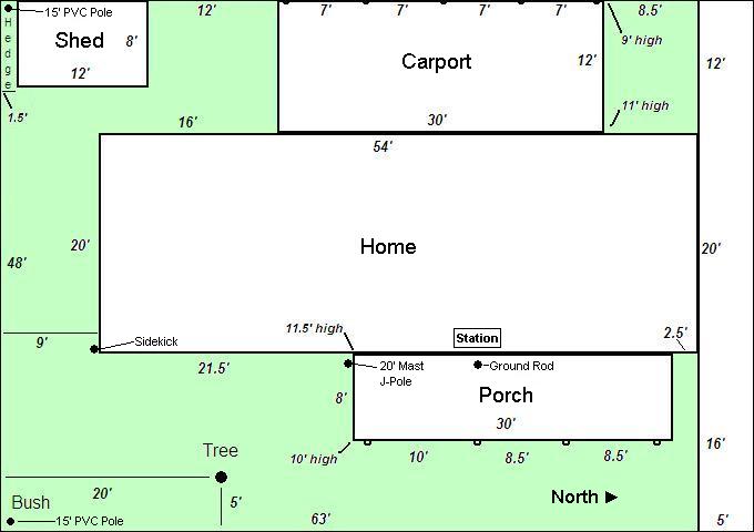
To start, I measured the property with its significant structures
and the antennas (Figure 2). Figuring the x,y,z coordinates from the
station ground point 0,0,0, these numbers were entered into the
program, along with the power source, load, wire radius and wire
connection data. (This process and guidelines are explained in
detail in the article "A Beginner's Guide to
Modeling with NEC"3, Cebik, LB, QST,
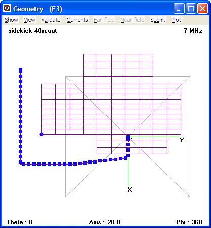
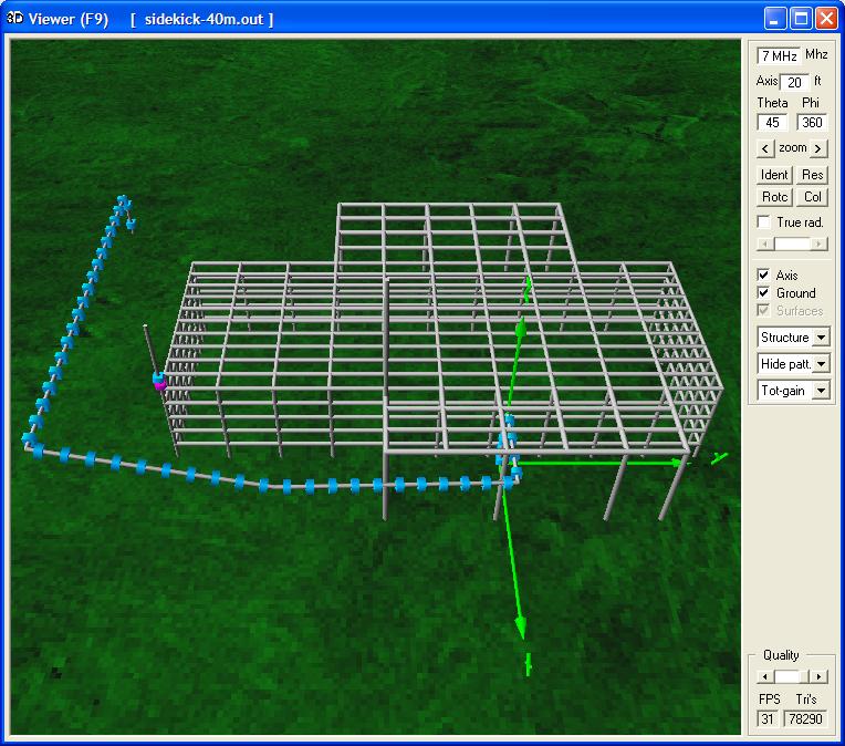
November 2000, pp. 35-38). Figures 3 and 4 show the program's
representation of the input file. The x-axis was oriented west-east,
the y-axis north-south and the z-axis from zenith to nadir. As the
proximity of the aluminum metal siding of the house in the near
field would exert a significant influence on antenna performance,
these surfaces were modeled as wire frames using 4nec2's Geometry
Builder utility. Trees and other non-metallic structures having a
lesser effect on antenna performance were ignored in the model. The
model ground was selected as "Real Ground" and "Good" quality. North
is toward the right in Figures 1 through 4.
|
|
|
|
|
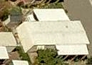
Fig. 1. Aerial photo of property (north is
right)
|
Fig. 2. Survey map of property
|
Fig. 3. 2-D model
|
Fig. 4. 3-D model
|
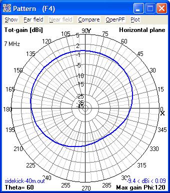
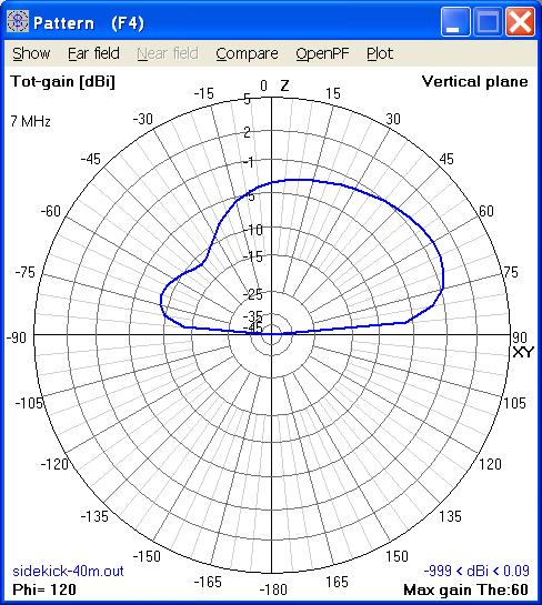
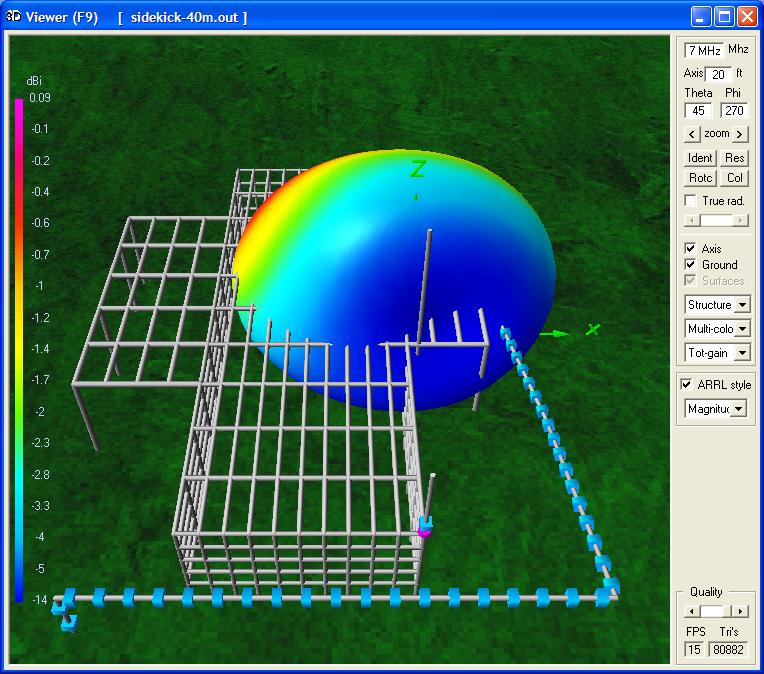
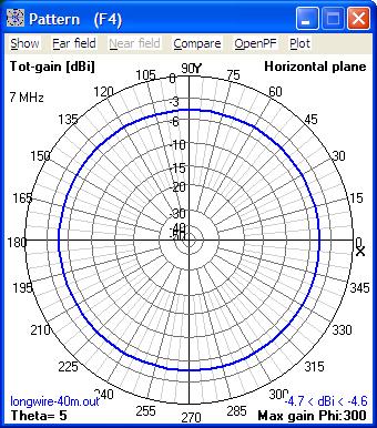
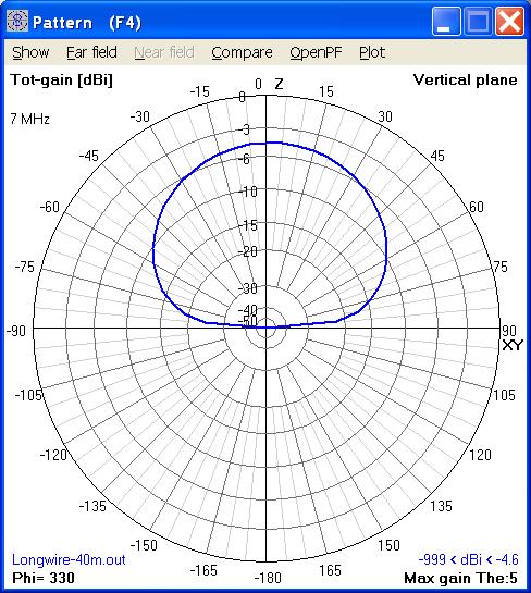
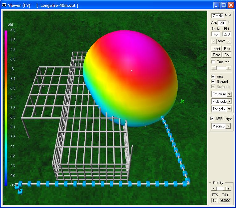
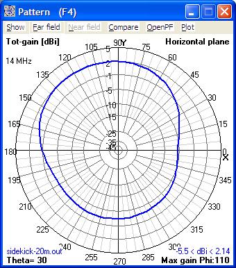
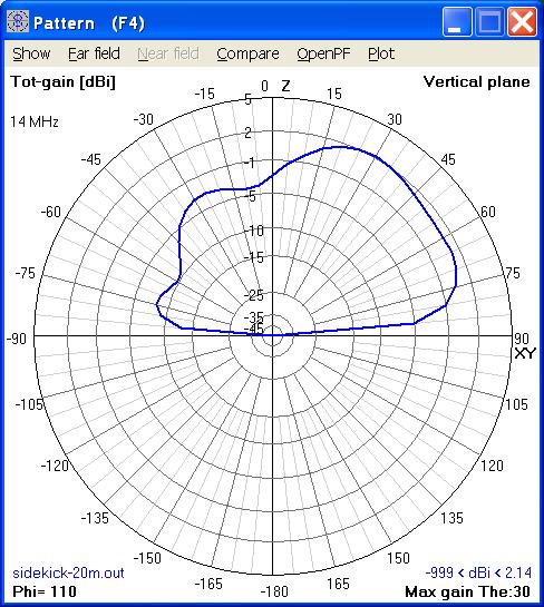
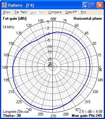
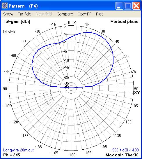
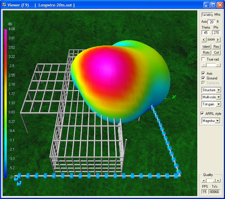
Figures 5 through 16 are the calculated far field radiation
patterns comparing the vertical antenna and the random wire
antenna on 7 and 14 MHz (North is at the top of all azimuth and
3-D patterns).
|
|
|
|
Fig. 5. Vertical 7 MHz azimuth pattern
|
Fig. 6. Vertical 7 MHz elevation pattern
|
Fig. 7. Vertical 7 MHz 3-D pattern
|
|
|
|
|
Fig. 8. Random wire 7 MHz azimuth pattern
|
Fig. 9. Random wire 7 MHz elevation pattern
|
Fig. 10. Random wire 7 MHz 3-D pattern
|
|
|
|
|
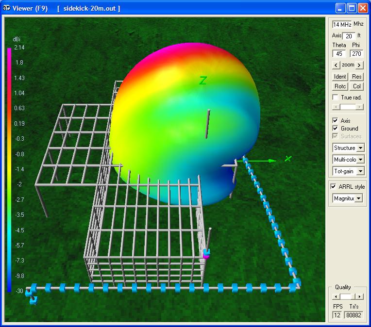
Fig. 11. Vertical 14 MHz azimuth pattern
|
Fig. 12. Vertical 14 MHz elevation pattern
|
Fig. 13. Vertical 14 MHz 3-D pattern
|
|
|
|
|
Fig. 14. Random wire 14 MHz azimuth pattern
|
Fig. 15. Random wire 14 MHz elevation
pattern
|
Fig. 16. Random wire 14 MHz 3-D pattern
|
Table 1 below lists the calculated major lobes of radiation, the
direction of the major lobe, and overall radiation
efficiency. The radiation efficiency is a measure of the
overall proportion of power that is radiated into space after
losses in the structure and the ground are subtracted.
Frequency
MHz
|
Vertical Antenna
|
Random Wire Antenna
|
Maximum
gain dBi
|
Lobe
direction(s)
|
Radiation
efficiency
|
Resistance
ohms
|
Reactance
ohms
|
SWR @
50 ohms
|
Maximum
gain dBi
|
Lobe
direction(s)
|
Radiation
efficiency
|
Resistance
ohms
|
Reactance
ohms
|
|
7 MHz
|
0.09
|
NNW
|
21.48%
|
16.2
|
0
|
3.08
|
-4.6
|
Omnidirectional
|
5.147%
|
182
|
-j87.1
|
|
14 MHz
|
2.14
|
NNW
|
27.28%
|
51.1
|
0
|
1.02
|
4.08
|
SSW
|
35.25%
|
497
|
+j962
|
Table 1. Comparison of vertical
and random wire antennas on 7 and 14 MHz
The calculated directionality of the vertical antenna corresponds
with the observed performance with nulls in the south and east
directions. From 65% to 95% of the transmitter power was
wasted in structure and ground losses.
DESIGNING A HORIZONTAL LOOP ANTENNA
MODEL
The desirable features of the new antenna were: low visibility from
the street, improved omnidirectionality, improved radiation
efficiency, operability on multiple bands (at least 7, 14, 21 and 28
MHz), broader bandwidth than the screwdriver vertical antenna to
allow some frequency changes within each band segment without
retuning, 100 watt power capacity, reduced sensitivity to local
noise, and removal of strong radio frequency fields away from the
interior of the home. In 1985, Fischer described a full wave
horizontal loop antenna (also known as a "Loop Skywire"4) as meeting these
requirements. With additional supports, the existing random wire
antenna could be extended to complete a 40 meter full wave loop, and
the feed point would be elevated above the roof. The loop antenna
would be fed with a balanced transmission line. Despite its
lower power capacity and higher dielectric loss and attenuation per unit length than
some coaxial cables, a short run of dual conductor speaker wire used
as a parallel transmission line is lighter, less visible, more
easily available and economical than coaxial cable.
Speaker wire is also very easily wound on a ferrite toroid core to
form a common mode choke or 1:1 current balun. Hall5,
Parmley6, and Wiesen7 have also discussed and
characterized the use of zip cords as transmission lines.
I chose to raise the feed point to the top of the 20 foot mast
that supported a VHF/UHF J-pole antenna. This additional height
was needed for the loop to clear the top of the tree in the
backyard. A rope and pulley would be used to raise and lower the
feed point for maintenance and antenna adjustments. A new 15 foot
PVC pole would be tied to a carport upright to support the fourth
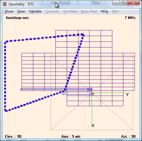
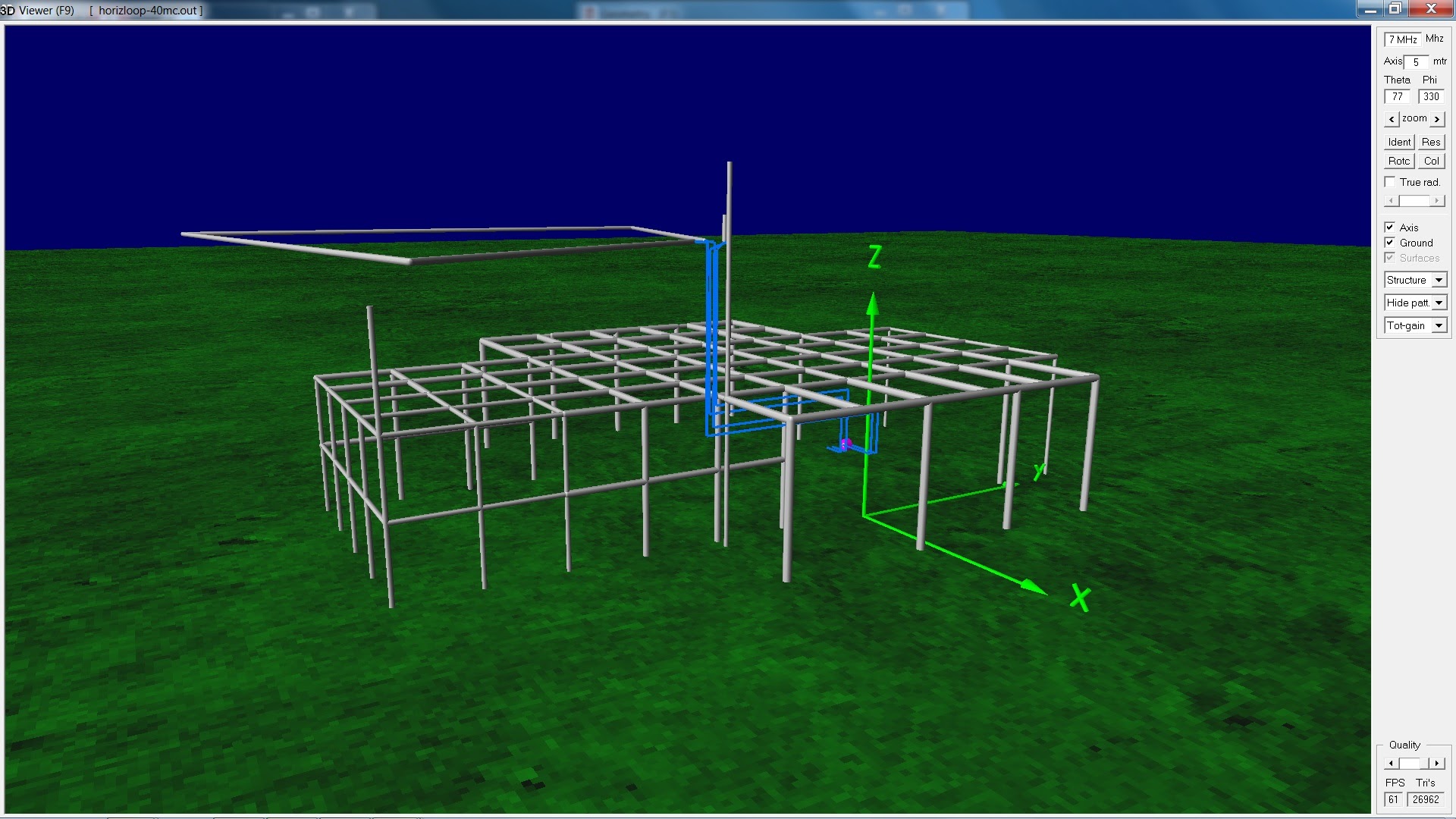
corner of the loop. The resulting loop geometry would be a
horizontal trapezoid with two sides sloping up to the feed point
(see Figures 17 and 18). In order to have a wire segment length on
the order of .05 wavelength on the highest frequency (28 MHz), 80
segments were required. To have all segments of nearly equal
length, the two sides nearest the feed point were given 18
segments each, and the far sides were given 22 segments
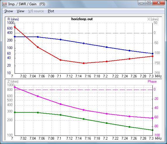
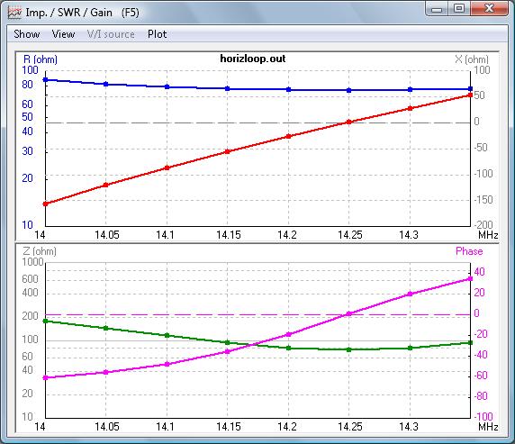
each. By trial and error, it was found that locating a
corner of the loop over the center carport upright yielded the
desired resonant frequencies in the 7 and 14 MHz bands (Figures 19
and 20). Download the NEC input file.
|
|
|
|
|
Fig. 17. Horizontal loop 2-D model
|
Fig. 18. Horizontal loop 3-D model
|
Fig.19. Reactance/resistance over 7 MHz
Resonance near 7.01 MHz.
|
Fig.20. Reactance/resistance over 14 MHz
Resonance at 14.25 MHz.
|
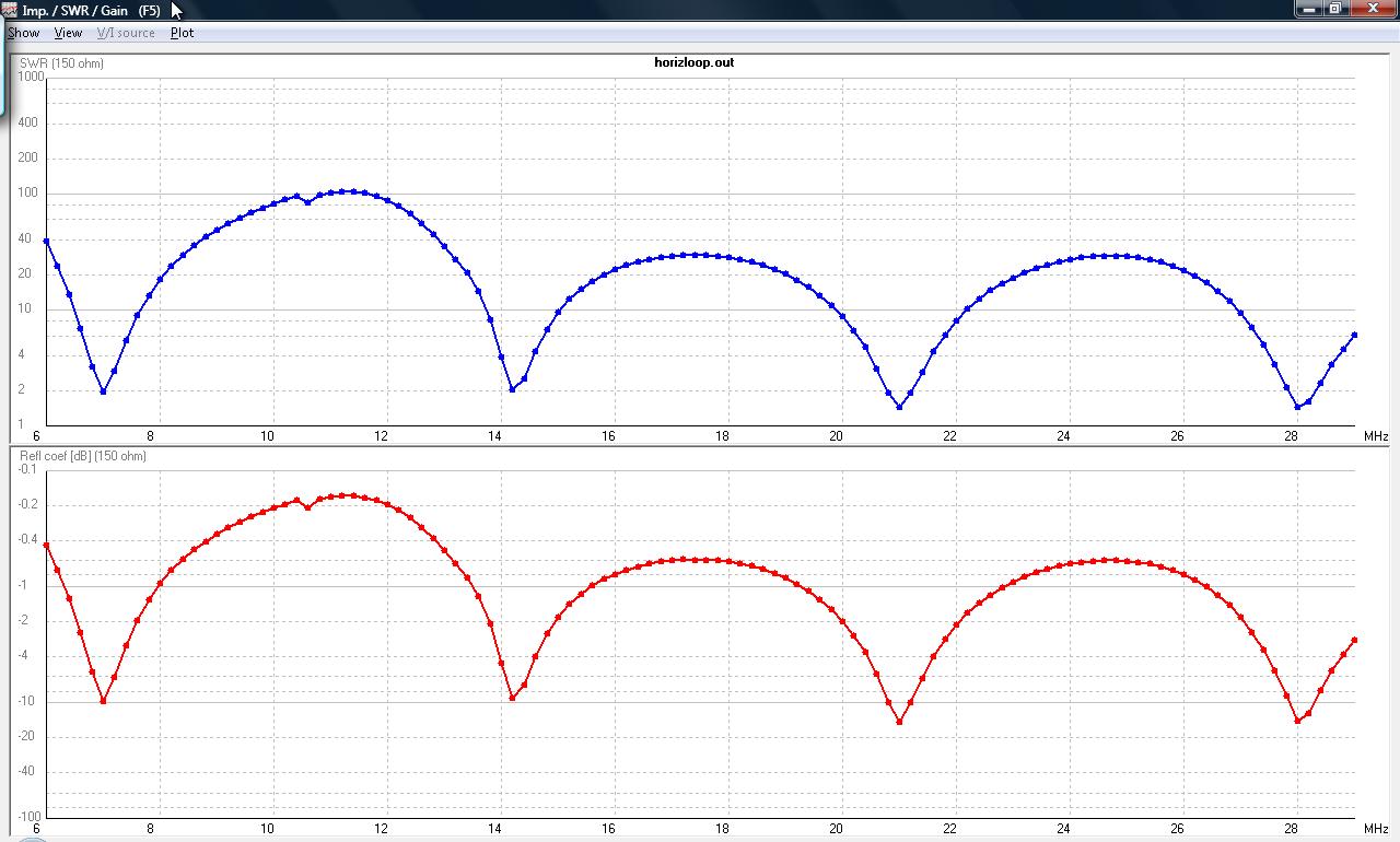
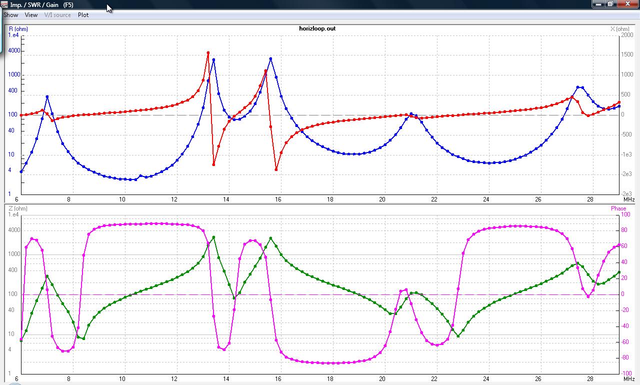
ANALYZING THE LOOP ANTENNA MODEL
The full range frequency sweep (Figures 21 and 22) predicted
resonances within the 7, 14, 21 and 28 MHz bands.
|
|
|
Fig. 21. Frequency sweep of SWR over 6-29
MHz
|
Fig. 22. Frequency sweep of reactance &
impedance over 6-29 MHz
|
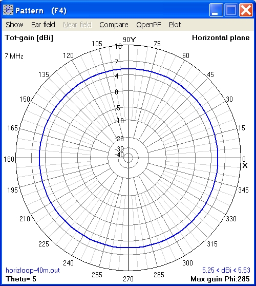
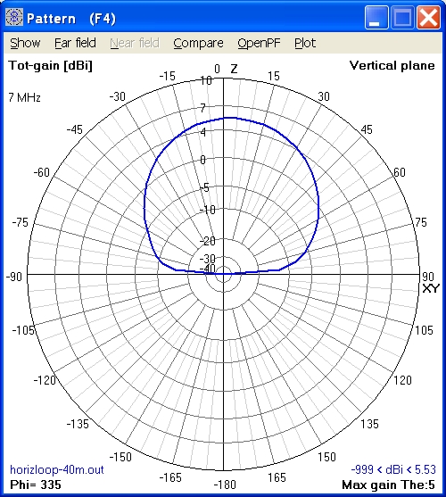
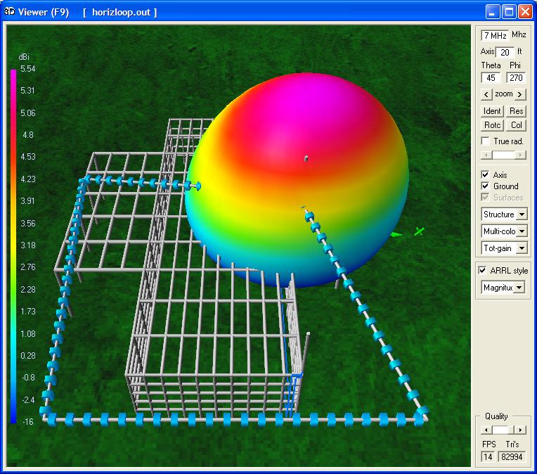
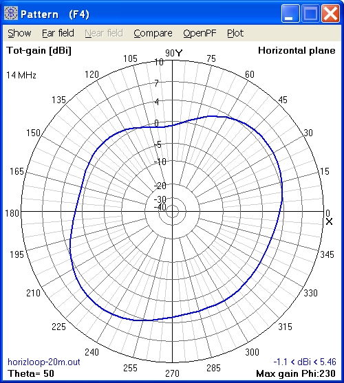
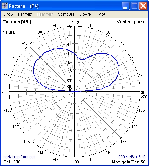
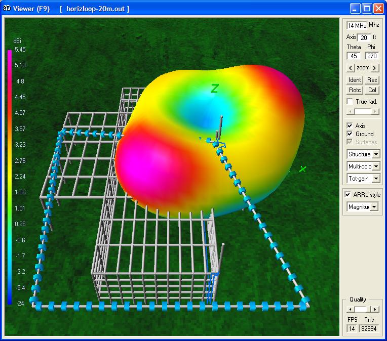
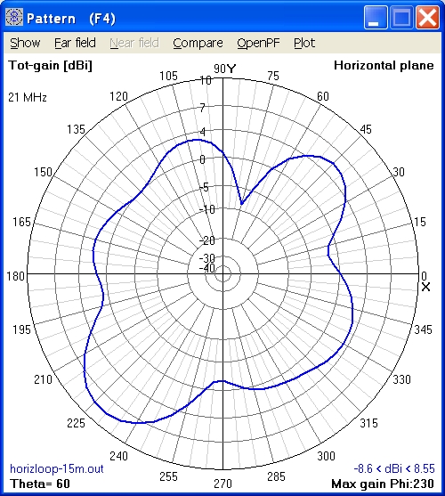
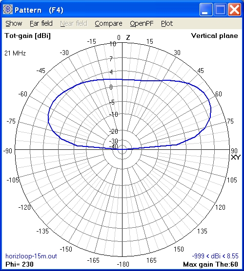
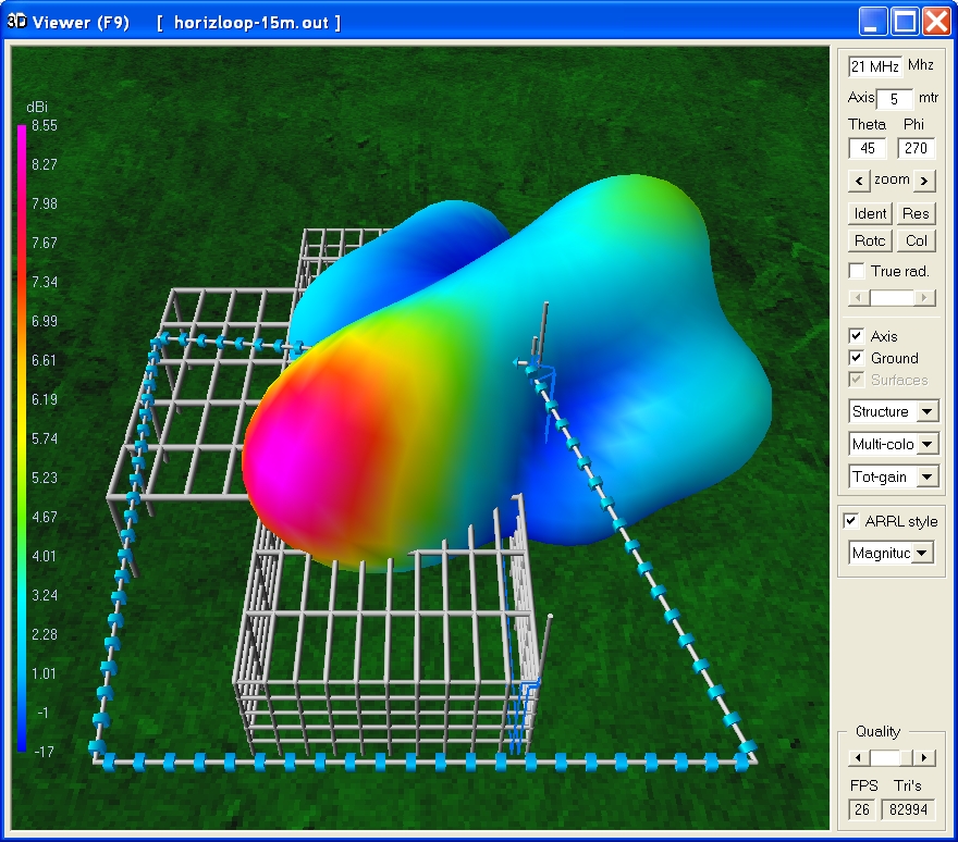
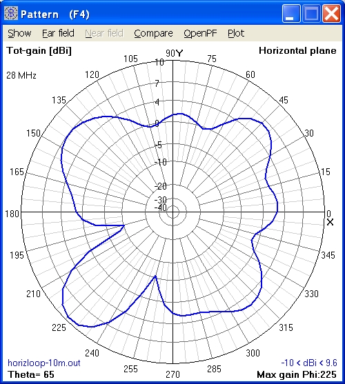
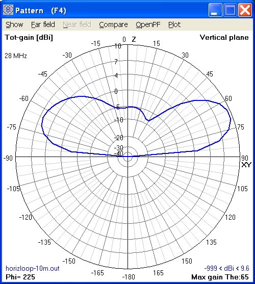
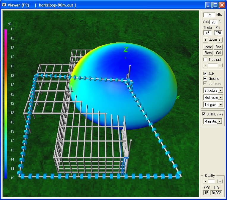
Figures 23 through 34 show the calculated far field radiation
patterns for the horizontal loop antenna on 7, 14, 21 and 28 MHz.
|
|
 |
|
Fig. 23. Loop 7 MHz azimuth pattern
|
Fig. 24. Loop 7 MHz elevation pattern
|
Fig. 25. Loop 7 MHz 3-D pattern
|
|
|
|
|
Fig. 26. Loop 14 MHz azimuth pattern
|
Fig. 27. Loop 14 MHz elevation pattern
|
Fig. 28. Loop 14 MHz 3-D pattern
|
|
|
 |
|
Fig. 29. Loop 21 MHz azimuth pattern
|
Fig. 30. Loop 21 MHz elevation pattern
|
Fig. 31. Loop 21 MHz 3-D pattern
|
|
|

|
|
Fig. 32. Loop 28 MHz azimuth pattern
|
Fig. 33. Loop 28 MHz elevation pattern
|
Fig. 34. Loop 28 MHz 3-D pattern
|
Table 2 below compares the calculated major lobes of radiation,
the direction of the major lobes, and overall radiation efficiency
of the vertical, random wire and horizontal loop antennas.
Frequency
MHz
|
Loop Antenna
|
Vertical Antenna
|
Random Wire Antenna
|
Maximum
gain dBi
|
Lobe
direction(s)
|
Radiation
efficiency
|
Maximum
gain dBi
|
Lobe
direction(s)
|
Radiation
efficiency
|
Maximum
gain dBi
|
Lobe
direction(s)
|
Radiation
efficiency
|
|
7 MHz
|
5.53
|
Omnidirectional
|
53.93%
|
0.09
|
NNW
|
21.48%
|
-4.6
|
Omnidirectional
|
5.147%
|
|
14 MHz
|
5.45
|
NW-NE-SW-SE
|
59.41%
|
2.14
|
NNW
|
27.28%
|
4.08
|
SSW
|
35.25%
|
Table 2. Comparison of
horizonal loop, vertical and random wire antennas
On 7 MHz, the loop antenna offered omnidirectionality with mostly
high angle radiation, 5.5 dB more maximum gain and over double the
radiation efficiency of the vertical antenna, and 10 dB more
maximum gain and 10 times the radiation efficiency of the random
wire antenna.. On 14 MHz, compared to the other antennas the
loop antenna offered near omnidirectionality, low angle of
radiation, up to 3.3 dB more maximum gain and up to twice the
radiation efficiency.
The random wire antenna was removed, and Table 3 compares the
4nec2 calculations for the horizontal loop antenna (SWR at the
feed line characteristic impedance of 114 ohms) with the vertical
antenna on all amateur radio high frequency bands.
Frequency
MHz
|
Loop Antenna
|
Vertical Antenna
|
Maximum
gain dBi
|
Lobe
direction(s)
|
Radiation
efficiency
|
Resistance
ohms
|
Reactance
ohms
|
Impedance
ohms
|
SWR @
114 ohms |
Maximum
gain dBi
|
Lobe
direction(s)
|
Radiation
efficiency
|
Resistance
ohms
|
Reactance
ohms
|
SWR @
50 ohms
|
|
1.8 MHz
|
-22*
|
Omnidirectional
|
0.158%
|
3.53
|
-j566
|
566
|
828*
|
N/A
|
N/A
|
N/A
|
N/A
|
N/A
|
N/A
|
|
3.5 MHz
|
-3.7*
|
Omnidirectional
|
8.561%
|
0.38
|
-j162
|
162
|
905*
|
-2.3
|
Omnidirectional
|
14.69%
|
6.17
|
0
|
8.11
|
|
5.3 MHz
|
3.55*
|
Omnidirectional
|
37.08%
|
1.13
|
-j47.4
|
47.4
|
118*
|
-0.6
|
NNW
|
18.06%
|
9.17
|
0
|
5.45
|
|
7 MHz
|
5.53
|
Omnidirectional
|
53.93%
|
287
|
+j34.1
|
289
|
2.56
|
3.79**
|
Omnidirectional
|
37.12%**
|
63.8
|
0
|
1.28
|
|
10.1 MHz
|
6.55*
|
Omnidirectional
|
63.82%
|
2.5
|
+j93.2
|
93.2
|
76.1*
|
0.77
|
NNE
|
25.65%
|
29.7
|
0
|
1.68
|
|
14 MHz
|
5.46
|
NW-NE-SW-SE
|
59.4%
|
84.1
|
-j152
|
174
|
4.27
|
2.06
|
NNW
|
27.46%
|
51
|
0
|
1.02
|
|
18.1 MHz
|
7.61*
|
NE-SW
|
71.22%
|
11.6
|
-j159
|
159
|
29.0*
|
2.79
|
NW
|
32.48%
|
62.4
|
0
|
1.25
|
|
21 MHz
|
8.55
|
NW-NE-SW-SE
|
67.91%
|
110
|
-j13.7
|
111
|
1.14
|
3.3
|
N
|
37.02%
|
64.9
|
0
|
1.3
|
|
24.9 MHz
|
7.8*
|
NW-NE-SW-SE
|
72.09%
|
7.73
|
+j106
|
106
|
27.5*
|
3.91
|
N
|
40.05%
|
81.5
|
0
|
1.63
|
|
28 MHz
|
9.6
|
NW-NE-SW-SE
|
69%
|
210
|
+j12.1
|
210
|
1.85
|
4.42
|
NW
|
42.91%
|
78.4
|
0
|
1.57
|
Table 3. 4nec2
calculations for horizontal loop and vertical antennas from
1.8 through 28 MHz
*High standing wave ratios were expected to cause increased
losses on frequencies other than 7, 14, 21 and 28 MHz.
**Replacing the random wire with the loop antenna significantly
increased the maximum gain and radiation efficiency of the
vertical antenna on 7 MHz where near field coupling induced
significant currents in and radiation from the loop antenna.
BUILDING THE LOOP ANTENNA
Here is a pictorial description of the materials used and the
construction of the loop antenna.
|
|
|
|
|
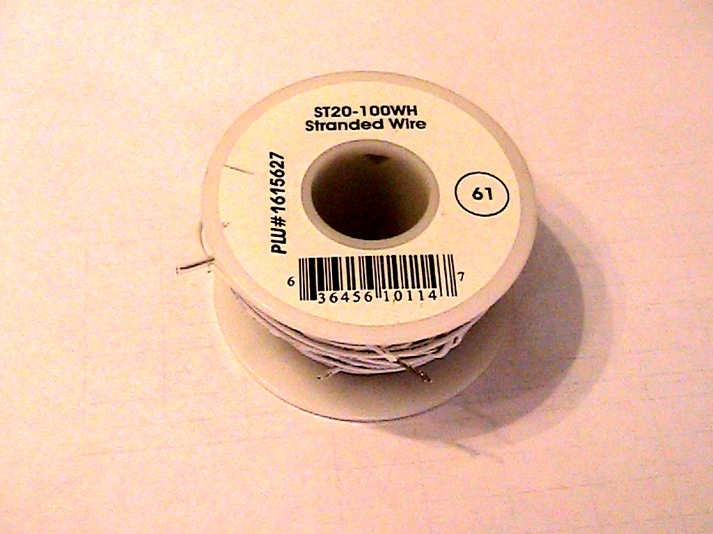
| The wire loop antenna is made of 140 feet of CTI-20
gauge insulated stranded wire. Cost $10. |
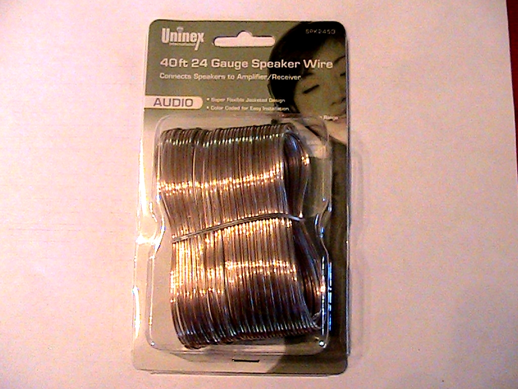
The balanced feed line was this 40' roll of 24 gauge
speaker wire. Later replaced with 18 gauge speaker wire. |
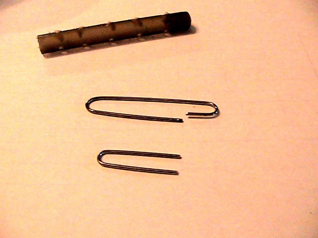
The feed point insulator is made from a paper clip and
half of a ball point pen barrel. UV exposure
degraded this plastic. Later replaced with a more
durable insulator.
|
Five holes are drilled in the pen barrel and the clip is
fashioned into an eye hook for the support rope. |
The feed point is half assembled. Wire nuts splice the
feed line to the ends of the loop antenna. |
|
|
|
|
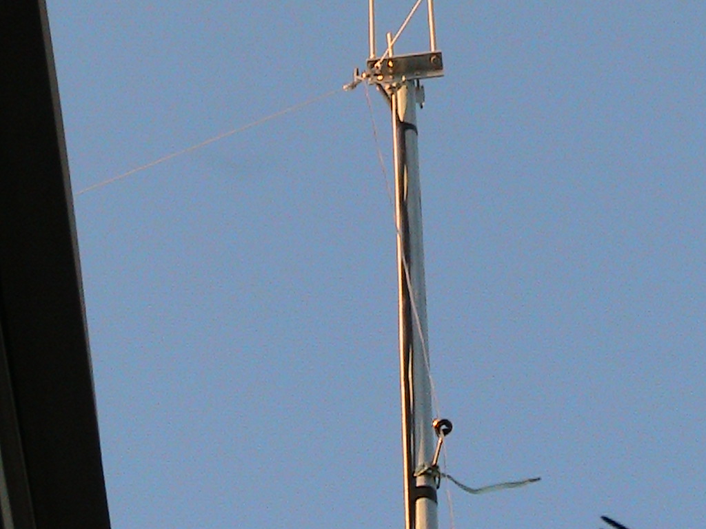
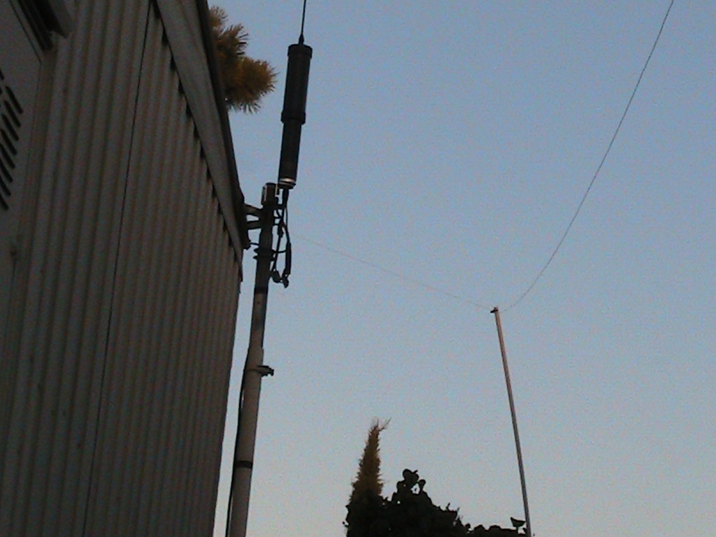
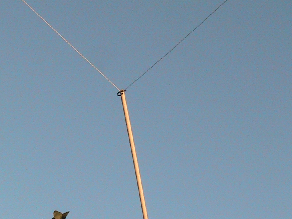
|
| This tie string tension pulley is mounted atop the mast
that supports the feed point with a machine screw eye
bolt. |
Here is the assembled feed point raised 20 feet to the
top of the supporting mast. |
Here is the southeast corner of the loop antenna. The
screwdriver antenna base is visible on the roof of the
house. |
At the corner supports, the loop wire passes through a
zip tie secured through a hole in the PVC pole. Later
replaced with 20 foot telescoping
fiberglass poles.
|
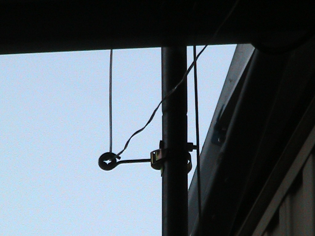
The feed line is suspended away from the mast with twin
lead standoff insulators. |
|
|
|
|
|
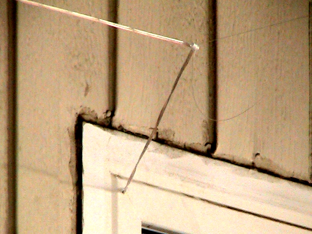
| A standoff insulator maintains the feed line (twisted
along its length) distance from the porch awning. |
A nylon monofilament suspends the feed line where it
bends to pass through the vinyl window frame. |
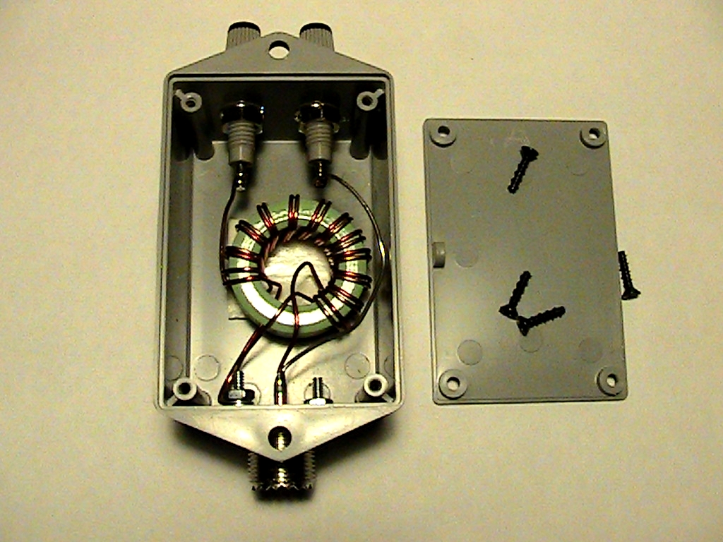
4:1 Ruthroff (voltage) balun matched the coax cable to
the balanced load.
Later replaced with 1:1 current
balun. |
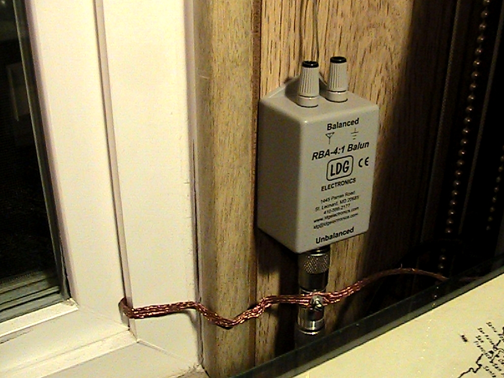
The feed line & balun are installed. The
copper braid exits the window to the ground rod. |
After the blinds are closed, the feed line and balun are
out of view. |
ADJUSTING AND MEASURING THE LOOP
ANTENNA
Given inaccuracies in the measurements and unaccounted environmental
influences on the antenna model, we expected to have to adjust the
wire length. A preliminary test showed the loop's fundamental
resonant frequency was 6850 kHz. Shortening the loop by
4 feet brought the SWR minima measured with a vector network
analyzer at the antenna feed point (Figure 35) close to those
predicted in Figure 21.
Ideally, antenna impedance measurements should be taken directly
at the antenna feed point. The data in Figures 35 through 37
were collected remotely with a Bluetooth connected miniVNA Pro vector
network analyzer connected directly to the antenna feed point.
Measurements with an unbalanced antenna analyzer, such as an
MFJ-259, at the feed point or through the balanced transmission
line must be taken through a 1:1 current balun. I built one
such balun by passing 12 turns of RG-174/U miniature 50 ohm cable
through a stacked pair of FT114-43 toroid cores and another one by
wrapping 30 turns of RG-174/U around a 4-3/4" x 3/8" ferrite rod
salvaged from a transistor radio (Figure 38). Either of
these gave comparable results.
| Horizontal Loop Antenna Parameters Measured
at Feed Point |

|
 |
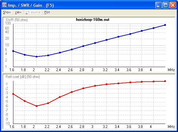
| Fig. 35. Standing Wave Ratio and Reflection Loss over
3-30 MHz |
Fig. 36. Resistance and reactance over 3-30 MHz |
 |

|
| Fig. 37. Impedance and phase over 3-30 MHz |
Fig. 38. Homemade 1:1 current baluns
|
Comparing these to the NEC model data in Figures 21 and 22,
the measured frequencies of SWR and impedance minima and points of
zero reactance at 7, 14, 21 and 28 MHz coincided with predicted
values. Note that frequency data obtained through a
transmission line will be skewed by impedance transformation.
An interesting finding was that the measurements were
significantly affected when the loading coil of the vertical
antenna was tuned to the same frequency at which the loop was
being measured. This effect was most prominent on 7 MHz and
decreased at the higher frequencies. This confirmed others'
observations that loop performance is affected by other resonant
objects within the near field of the antenna. For this
reason, the loading coil on the Sidekick vertical antenna was set
to minimum inductance during all measurements of the loop antenna.
ON THE AIR TESTING
On frequencies below 7 MHz, the loop antenna often
provided clearer reception of signals with lower noise
levels, although signal reports from other stations showed
that the vertical antenna was the more efficient
radiator. Later, received noise
levels on both antennas were quantitatively compared.
On 7 MHz received sky wave signals were predominantly up
to 12 dB stronger on the loop, with few signals favored by
the vertical antenna. Above 7 MHz received and
transmitted sky wave signals were predominantly stronger
on the loop antenna.
In the week after the loop antenna was erected on 11
September, 2010, my
online
log recorded solid contacts on 40 meters with
stations in the eastern USA, Australia, Brazil,
Guatemala, Japan and South Korea, areas that I could
rarely contact with my previous antennas. Within
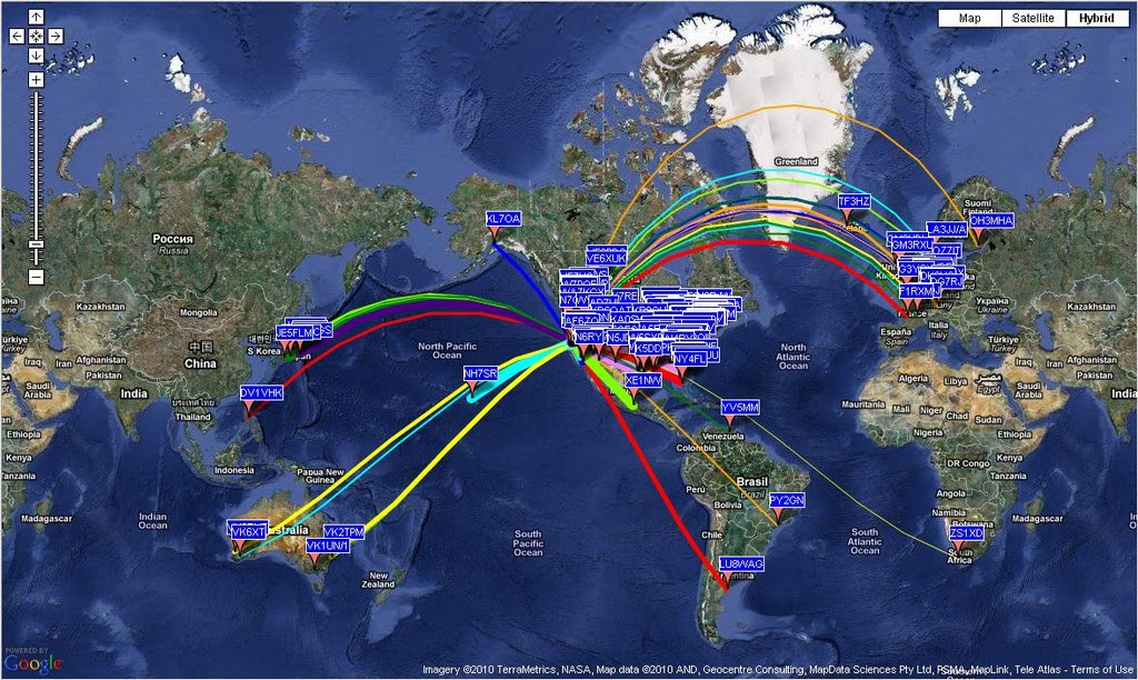
12 hours on 10 November 2010, the horizontal loop
antenna yielded confirmed contacts on 6 continents using
5 watts with WSPR mode
on 7 and 14 MHz. Starting in January 2011 WSPR
data was used for further analysis
of antenna performance.8
Comparisons between the antennas in contacts with local
stations via ground wave were variable, favoring either
the vertical antenna or the loop antenna depending on
polarization and antenna directivity.
|
|
|
Fig. 39. 6 continents in 12 hours using 5
watts WSPR mode on 7 & 14 MHz.
|
ADDENDUM - 07 October 2010 - The Horizontal Loop as a Top
Loaded Vertical Antenna
ANALYZING THE LOOP AS A TOP LOADED
VERTICAL ANTENNA
Others have reported using the horizontal loop antenna below the
design frequency by feeding both sides of the feed line tied
together against ground. This would, in effect convert the
loop and feed line into a random length top-loaded vertical
antenna. The full range frequency sweep (Figures 40 and 41)
predicted resonance outside the 1.8 and 3.5 MHz bands.
|
|
|
Fig. 40. Frequency sweep of SWR over 1.6-4.2
MHz
|
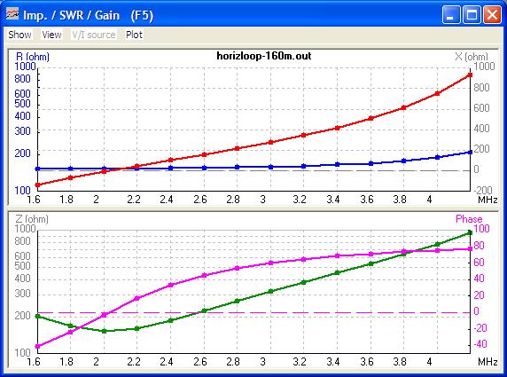
Fig. 41. Frequency sweep of reactance &
impedance over 1.6-4.2 MHz
|
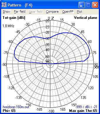
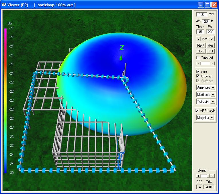
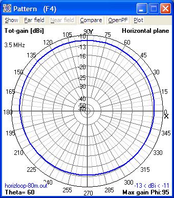
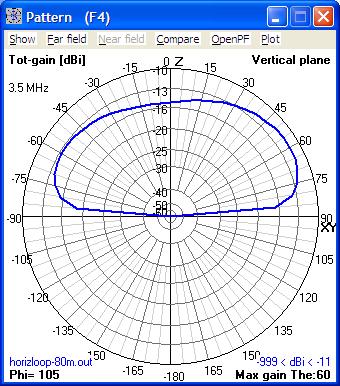
Figures 42 through 47 show the calculated far field radiation
patterns for the antenna used in this manner on 1.8 and 3.5 MHz.
|
|
 |
|
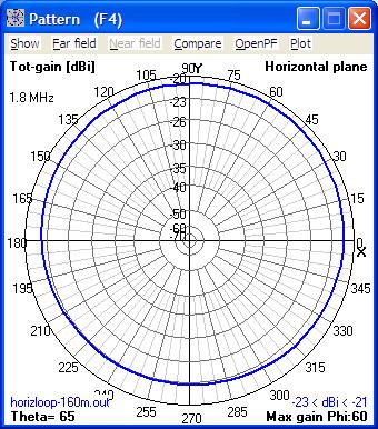
Fig. 42. Loop as vertical 1.8 MHz azimuth
pattern
|
Fig. 43. Loop as vertical 1.8 MHz elevation
pattern
|
Fig. 44. Loop as vertical 1.8 MHz 3-D
pattern
|
|
|
|
|
Fig. 45. Loop as vertical 3.5 MHz azimuth
pattern
|
Fig. 46. Loop as vertical 3.5 MHz elevation
pattern
|
Fig. 47. Loop as vertical 3.5 MHz 3-D
pattern
|
Table 4 below shows the calculated low gain and overall radiation
efficiency of the horizontal loop antenna used in this manner.
Frequency
MHz
|
Top Loaded Vertical Antenna
|
Maximum
gain
|
Lobe
direction(s)
|
Radiation
efficiency
|
Resistance
ohms
|
Reactance
ohms
|
|
1.8 MHz
|
-21 dBi
|
Omnidirectional
|
0.232%
|
152
|
-j68.3
|
|
3.5 MHz
|
-11 dBi
|
Omnidirectional
|
2.187%
|
167
|
+j462
|
Table 4. Gain and radiation
efficiency of loop antenna as vertical
ON THE AIR TESTING
As 4nec2 predicted that the antenna would present
non-resonant load, the transmitter was connected to it through the
MFJ-949B antenna tuner without the balun. The tuner was able
to present a 50 ohm non-reactive load to the transmitter, which
delivered the full rated 100 watts. Reception was adversely
affected by radio frequency interference from appliances, and a
significant transmitted radio frequency field inside the station
caused intermittent operation of a computer, touch lamps and
television. Despite the predicted low radiation efficiency, my
initial contact on 3.5 MHz was reported as S9 signal strength at
K2LMQ, 459 miles away in Kingman, AZ on 7 Oct 2010 at 0502 UTC.
Update - 04 December 2010 - Antenna Feed System Improvements
Described in detail separately in Zip Cord Transmission Lines and
Baluns9
In December 2010, the 24 AWG transmission line was
replaced with lower loss 18 AWG speaker wire (Figure 48),
common mode chokes were added (Figure 49) and the 4:1
voltage balun was replaced with a 1:1 current balun
(Figure 50) in order to reduce the antenna feed system
noise and attenuation.
In December 2017, to accommodate an increase in transmitter
power to 500 watts, I wound a new 1:1 current balun on two stacked
FT240-43 ferrite cores and replaced the speaker wire feed line with
300 ohm Ladder Line. The latter also very
significantly decreased the feed line dielectric losses on the WARC bands
and on frequencies above 14 MHz.
Figure 60 shows the present station antenna
configuration. With the 1:1 current balun on the
output of the antenna tuning unit and the total
transmission line length adjusted to 1/2
electrical wavelength at 7 MHz, the impedance presented
was well within the range of the tuner on all frequencies
3.5, 7, 10, 14, 18, 21, 24 and 28 MHz.

Figure 48. Pfanstiehl
18AWG AS-18/50Z
Speaker Wire
|

Figure 49. 1:1 choke at
feed point - 11 turns on
FT114-43 core
|

Fig. 50. 1:1 current balun made of RG-174/U
coaxial cable on two FT114-43 toroid cores
|

FT240-43 1:1 current balun |

Ferrites on Ladder Line |
Update - 28 August 2013 - 40 Meter Loop
Antenna Transmission Line Optimization for 80 Meters and WARC
Bands
As seen above in Figures 35 and 36, the 40 meter full wave loop
antenna presents a non-reactive load on its fundamental resonant
frequency and harmonics thereof, but between these frequencies high
impedance presents matching problems at the transmitter end of
the transmission line. In addition, the impedance transforming
properties of random transmission line lengths skew the resonant
frequencies seen at the transmitter end of the feed line.
The vector network analyzer measurements at Figures 51 and 52
below demonstrate this effect measured at the transmitter end of
the original random length 37.9 foot zip cord transmission line.
Not only were the resonant frequencies skewed outside of the
desired frequency bands, but the high impedance presented to the
transmitter on the 80 meter and the 30, 17 and 12 meter "WARC"
bands rendered impedance matching problematic at those
frequencies.
Figures 53 and 54 demonstrate the effect of lengthening the zip
cord transmission line to an electrical quarter-wavelength at 3.5 MHz
(51 feet). This eliminated skewing of the natural resonant
frequencies of the loop antenna at its natural fundamental and
harmonic frequencies. Also, the impedance transforming
characteristics of this transmission line at frequencies where it
is also an odd multiple of a quarter-wavelength (3.5, 10.5, 17.5,
and 24.5 MHz) transformed the loop antenna's high impedance at
those frequencies to a low impedance, eliminating high RF voltage
on and facilitating transmitter matching with my LDG Z-11Pro II
automatic antenna tuning unit with an attached 1:1 current balun
on 3.5 MHz and the WARC bands.
The principle of the 7 MHz full-wave loop operation on 3.5 MHz
may be conceptualized by comparison with the HO loop, or halo
antenna—a half-wave open loop antenna popular on VHF frequencies.
The halo antenna is essentially a horizontal half-wave dipole with
its elements curved to form an open-ended circular loop to provide
a nearly omnidirectional radiation pattern. The halo antenna is
typically fed at its low impedance center point, while its open
ends exhibit high impedance. By analogy, the 7 MHz full-wave loop
operates on 3.5 MHz as a half-wave halo antenna fed across its
high impedance open ends. In this case, the impedance transforming
characteristic of a 1/4 wavelength transmission line assists in
coupling the high impedance antenna to the low 50 ohm impedance of
the transmitter. This situation repeats at frequencies where
the loop antenna is an odd multiple of a quarter-wavelength, that is,
at 10.5, 17.5 and 24.5 MHz, near the "WARC" frequency bands.
The 100 and 300 ohm lines are preferable to 450 and 600 ohm lines
for this application. As can be seen in Figure 37,
the measured loop feed point impedance varies between 80 and 350 ohms at its resonance
points and between 800 and 1800 ohms at the midpoint peaks between
resonance. For a quarter wavelength transmission line, the
impedance seen by the transmitter (Z) is given by Z = Z02
/ Zant, where Z0 is the characteristic
impedance of the transmission line and Zant is the
antenna impedance. Figures 55 and 56 compare these impedance
transforming characteristics for 100 ohm and 450 ohm feed lines.
The 100 ohm feed line transforms the impedance to 6 to 125 ohms at
the transmitter, within the range of most antenna tuning units.
However, the higher impedance feed line renders an impedance range of 110 to
2500 ohms at the transmitter, values that exceed the operating
range and safe voltage ratings of many antenna tuners.
See more graphic analysis at Google Photos.
Horizontal Loop Antenna Parameters Measured
at Transmitter End of Feed Line over 3 to 30 MHz
|
 |

|
| Fig. 51. Standing Wave Ratio and Reflection Loss -
Random 37.9' feed line |
Fig. 52. Resistance and Reactance - Random 37.9' feed
line
|
") |
")
|
Fig. 53. Standing Wave Ratio and Reflection Loss - 51'
feed line (0.5λ @ 7 MHz)
|
Fig. 54. Resistance and Reactance - 51' feed line
(0.5λ @ 7 MHz)
|
Impedance
Transforming Characteristics of 100 and 450 ohm 1/4 Wave
Transmission Lines
|
 |
 |
Fig. 55. A 100 ohm feed line transforms the antenna
impedance to 6 to 125 ohms
at the transmitter, within the range of most antenna
tuning units. |
Fig. 56. A 450 ohm ladder line renders an impedance
range of 110 to 2500 ohms
at the transmitter, exceeding the safe operating range of
most antenna tuners. |
NOISE LEVELS
The received noise levels with the loop antenna and the Sidekick
vertical antenna were compared using a FlexRadio 3000 receiver set
to a 1 kHz passband on 3 February 2011 at 0400Z. The MFJ-949B
antenna tuner was adjusted for 1:1 standing wave ratio through the
parallel line 1:1 balun for each measurement with the loop antenna,
and the antenna loading coil was adjusted for minimum standing wave
ratio for each measurement with the vertical antenna. Table 5
lists the noise levels within 1 kHz and their conversion to the
standard dBm/Hz values and S units within a 3 kHz passband.
These levels represent a composite of atmospheric noise and local
man-made noise that vary with season and time of day.
Frequency
MHz
|
Loop antenna noise
|
Vertical antenna noise |
|
dBm/kHz
|
dBm/Hz
|
S units/3 kHz
|
dBm/kHz
|
dBm/Hz
|
S units/3 kHz
|
|
1.8 MHz
|
-114
|
-144
|
3
|
-100
|
-130
|
5.3
|
|
3.5 MHz
|
-113
|
-143
|
3.1
|
-106
|
-136
|
4.3
|
|
5.3 MHz
|
-112
|
-142
|
3.3
|
-108
|
-138
|
4
|
|
7 MHz
|
-108
|
-138
|
4
|
-108
|
-138
|
4
|
|
10.1 MHz
|
-115
|
-145
|
2.8
|
-105
|
-135
|
4.5
|
|
14 MHz
|
-109
|
-139
|
3.8
|
-113
|
-143
|
3.1
|
|
18.1 MHz
|
-117
|
-147
|
2.5
|
-112
|
-142
|
3.3
|
|
21 MHz
|
-116
|
-146
|
2.6
|
-118
|
-148
|
2.3
|
|
24.9 MHz
|
-126
|
-156
|
1
|
-120
|
-150
|
2
|
|
28 MHz
|
-125
|
-155
|
1.1
|
-121
|
-151
|
1.8
|
Table 5. Noise levels at receiver
As expected, the noise levels decreased with increasing
frequency. The noise levels were comparable on the loop
antenna and the vertical antenna on 7, 14, 21 and 28 MHz.
The loop yielded lower noise and lower received signal strengths
on 1.8 & 3.5 MHz and the WARC bands probably due to losses
associated with high line SWR on the speaker wire there,
and to the low radiation efficiency of the 40m loop on frequencies below 7 MHz.
Although the vertical antenna was the more efficient radiator below
7 MHz, the loop antenna yielded an average 10 dB better signal to noise
ratio on received signals below 7 MHz. This difference is likely due to:
coupling of radio frequency noise generated by home electronics
into the aluminum siding that serves as the counterpoise half of the
vertical antenna; and to the relative insensitivity of the horizontal loop
at the lower frequencies to the low elevation angles at which radio
frequency noise sources predominate.
The common mode signal and noise rejection were tested by
shorting both sides of the balanced feed line together and
observing for quieting of the receiver. Among the baluns, common
mode signal rejection was greatest in the current baluns and least
in the 4:1 voltage balun. At 3.5 MHz, the 4:1 voltage balun
showed no measurable rejection of common mode noise at all.
The toroid current baluns with their increased common mode signal
rejection also improved reception in the low frequency and medium
frequency ranges that were previously covered by strong
intermodulation products from nearby medium frequency AM broadcast
stations.
UPDATE - 09 Dec 2017 - Ladder Line Installed
The 18AWG speaker wire transmission line performed acceptably
at power levels up to 100 watts and on 7 and 14 MHz where the standing
wave ratio was under 3:1 and the dielectric loss was acceptable. However,
the dielectric loss was increasingly high above 14 MHz and with the high
feed line SWR on 80m and the WARC bands.
The acquisition of a 500 watt amplifier required replacement of the 18AWG
speaker wire feed line. A 17m (54 foot) length of JSC-1320 stranded copper
300 ohm Ladder Line was determined to be an electrical 0.25λ length at 3.5 MHz.
Television twin lead type standoff insulators served to route the wire to the 40 meter
full wave horizontal loop antenna. Since parallel transmission lines must be routed
several diameters away from other conductors, the excess length of the Ladder Line
was loosely coiled and suspended on a rope. Photo album
Ladder Line exhibits low dielectric loss regardless of high feed line SWR. Using a feed line of an electrical quarter wavelength for 3.5 MHz offers the benefit of transforming the loop's very high feed point impedance at 3.5, 10.1, 18, and 25 MHz to a low impedance at the transmitter end that is within the matching range of my antenna tuning unit. Although a full-sized 80m loop would be more efficient, this arrangement allows me to operate on 3.5 MHz and the WARC bands with the 40 meter loop that fits in my smaller available space. Here is an interactive chart of the SWR measured at the transmitter end of the feed line.
In order to increase its power capacity, the old FT140-43 ferrite choke balun was replaced with nine turns of 18AWG
speaker wire on two stacked FT240-43 toroid cores.
Here is an interactive chart of the common mode impedance of the balun.
I placed several Bluecell 13mm clip-on ferrite cores over the feed point end of the 300 ohm ladder line as a common mode choke (similar to a W2DU balun).
Its purpose is to help suppress undesired common mode current on the transmission line that would be caused by the asymmetric environment of the horizontal loop antenna. Photo album
Replacing the speaker wire with 300 ohm Ladder Line yielded an average 10 dB increase in signal to noise ratio of 3.5 MHz WSPR spot reports at KR6ZY.
This demonstrates the significantly lower loss that the Ladder Line exhibits under the high feed line SWR condition on 3.5 MHz.
The change from speaker wire transmission line to the 300 ohm Ladder Line also yielded a significant increase in number of 80m WSPR spot reports over 1800 km distance as shown on Distance vs. Date chart after 10 DEC 2017.
 |
 |
|
|
 > > |
| 17m (54 feet) of 300 ohm Ladder Line |
SWR at the transmitter end of the feed line |
FT240-43 1:1 current balun |
Clip on ferrites at feed point |
Ladder Line raised SNR by 10 dB on 3.5 MHz |
 UPDATE -
07 June 2011 - Loop Antenna
Raised
UPDATE -
07 June 2011 - Loop Antenna
Raised
In June 2011, the far corners of the loop antenna were raised with
green Jackite telescoping
fiberglass poles from 15 feet (4.6 m) to a height of 20 feet
(6.1 m) above ground so that the entire loop antenna would be in the
same horizontal plane as the feed point with the expectation that it
would increase efficiency by decreasing signal absorption by the
house structure and the ground. Jackite poles were selected as
they are lightweight, economical, adequate to support small gauge
wire, and superior in rigidity and aesthetic appearance to PVC
poles. The new NEC files are listed in
the appendix.
Table 6 compares the calculated maximum gain, gain at 15° elevation
(low angle for long distance propagation) and at 90° elevation (high
angle for NVIS short distance propagation) in the same direction,
and radiation efficiency for Sidekick screwdriver vertical antenna
with the loop antenna at the two different heights. The WSPR
column is an estimation of the overall effective radiated power at
each frequency for the WSPR transmitter with a nominal power output
of 5 watts, line attenuation of 35 feet of transmission line from Zip Cord Transmission Lines and Baluns9
(not including losses due to impedance mismatch), and radiation
efficiency of the loop antenna at 20 feet, .
Total ERP(W) = P(W) × 10-(attn(dB)/10)
× Rad. eff.(%)
Before
7 June 2011
|
After 7
June 2011
|
Frequency
MHz
|
Loop Antenna @ 15' (4.6 m)
|
Sidekick
Screwdriver Vertical Antenna |
Loop Antenna @ 20' (6.1 m)
|
Sidekick Screwdriver Vertical Antenna
|
Maximum
gain dBi
|
Gain-dBi
@15°elev.
|
Gain-dBi
@90°elev.
|
Radiation
eff. %
|
Maximum
gain dBi |
Gain-dBi
@15°elev |
Gain-dBi
@90°elev |
Radiation
eff. % |
Maximum
gain dBi
|
Gain-dBi
@15°elev. |
Gain-dBi
@90°elev. |
Radiation
eff. %
|
WSPR
Est.Total
ERP (W) |
Maximum
gain dBi |
Gain-dBi
@15°elev |
Gain-dBi
@90°elev |
Radiation
eff. % |
|
1.8
|
-23
|
-28.3
|
-25.6
|
0.12
|
|
|
|
|
-18
|
-25.5
|
-18.5
|
0.39
|
0.02
|
|
|
|
|
|
3.5
|
-4.4
|
-14.3
|
-4.37
|
7.09
|
-3.3
|
-4.03
|
-14.9
|
10.8
|
-1.2
|
-10.6
|
-1.17
|
14.4
|
0.57
|
-3.4
|
-4.05
|
-14.2
|
10.7
|
|
5.3
|
3.69
|
-6.7
|
3.65
|
37.4
|
-1.2
|
-2.1
|
-11.1
|
14.6
|
5.13
|
-6.74
|
5.11
|
51.0
|
|
-1.2
|
-2.15
|
-10.1
|
14.7
|
|
7
|
5.73
|
-4.67
|
5.65
|
56.1
|
4.54
|
-2.59
|
4.31
|
45.6
|
6.62
|
-7.17
|
6.58
|
66.5
|
2.4
|
1.8
|
-6.07
|
1.79
|
34.4
|
|
10.1
|
6.55
|
-2.02
|
6.11
|
64.8
|
0.85
|
-1.62
|
-0.13
|
24.7
|
7.03
|
-3.46
|
6.73
|
72.4
|
2.4
|
0.64
|
-2.12
|
-0.455
|
24
|
|
14
|
5.59
|
0.77
|
-2.01
|
61.3
|
3.76
|
-4.08
|
2.07
|
31.5
|
5.42
|
1.17
|
-3.8
|
68.3
|
2.1
|
2.68
|
-4.0
|
1.21
|
28.8
|
|
18.1
|
7.7
|
0.91
|
4.22
|
75.2
|
3.49
|
-1.12
|
-0.62
|
32.9
|
7.74
|
3.85
|
4.88
|
80.0
|
2.3
|
3.09
|
-0.85
|
-1.1
|
32.4
|
|
21
|
8.2
|
4.64
|
4.29
|
69.4
|
4.13
|
-1.44
|
1.07
|
36.9
|
9.24
|
6.26
|
5.3
|
78.2
|
2.2
|
3.7
|
-1.51
|
0.25
|
37.1
|
|
24.9
|
9.02
|
6.98
|
-3.69
|
72.1
|
4.22
|
0.37
|
1.19
|
41.3
|
9.65
|
8.08
|
-2.29
|
79.4
|
2.1
|
4.05
|
0.68
|
1.05
|
42.0
|
|
28
|
10.1
|
8.47
|
-2.93
|
68.2
|
5.28
|
2.17
|
2.53
|
46.4
|
11.4
|
10.5
|
2.51
|
74.4
|
1.9
|
4.74
|
2.15
|
1.52
|
45.4
|
50
|
10.0
|
10.0
|
-9.88
|
68.8
|
|
|
|
|
10.2
|
10.2
|
-9.53
|
70.8
|
1.4
|
|
|
|
|
Table 6.
4nec2 calculations for the Sidekick screwdriver vertical
antenna with the horizontal loop antenna at 15 feet and at 20
feet height above ground

|

|

|
Figure
57. NVIS Gain - Horizontal Loop vs. Vertical
|
Figure
58. Low Angle Gain - Horizontal Loop vs. Vertical
|
Figure
59. Radiation Efficiency - Horizontal Loop vs.
Vertical
|
With the horizontal loop antenna at this increased height above
ground, the modeling program predicted increases in radiation
efficiency on all frequencies and overall increases in gain at
both low and high elevation angles. Figures 57 through 59
compare the performance of the horizontal loop antenna against the
vertical screwdriver antenna. The loop antenna yielded
greater gain at the desired high radiation angles (near vertical
incident skywave or NVIS) for short distance paths on frequencies
below 14 MHz and at greater gain at low radiation angles as
desired for long distance paths on and above 14 MHz. The
loop antenna had significantly superior radiation efficiency on
all frequencies above 3.5 MHz.
CONCLUSION
Computer antenna modeling was useful in significantly
improving my station antenna performance. Adding some
wire and supports converted an inefficient random wire
antenna into a much more efficient full wave horizontal loop
antenna. The $15 spent for the loop antenna wire, feed line
and balun yielded significantly superior results to the
screwdriver antenna which cost $450. Compact antennas
like the Sidekick screwdriver vertical compromise
performance but have their applications for their
portability and when space is especially limited, as on a
vehicle.
ACKNOWLEDGEMENTS
Many thanks to Dutch engineer Arie Voors for sharing his
excellent 4nec2 antenna modeling
program with the radio amateur community, Magnus
Beischer, Don Lucas, Matt Pyne for their freeware TinyCAD
program used to draw the schematic diagram, Dan
Maguire for the Transmission Line Details
program, and to Larry Sutter, WD6FXR, who
very graciously permitted me the use of his MFJ-269 antenna
analyzer for this project.
REFERENCES
- "Computer Assisted Low Profile
Antenna Modeling I", Milazzo, C, KP4MD, 13 June
1998.
- 4nec2 antenna
modeling software, Voors, A.
- "A Beginner's Guide to
Modeling with NEC", Cebik, LB, W4RNL, QST,
November 2000, pp. 35-38.
- "The
Loop Skywire", Fischer, D, W0MHS, QST, November
1985, pp. 20-22.
- "Zip
Cord Antennas - Do They Work?", Hall, J, K1TD,
QST, March 1979, pp. 31-32.
- "Zip
Cord Antennas and Feed Lines For Portable
Applications", Parmley, W, KR8L, QST, March 2009,
pp. 34-36.
- "Portable
Antenna Notes", Wiesen, R, WD8PNL
- "Comparative Antenna Analysis with
WSPR", Milazzo, C, KP4MD, 13 January 2011.
- "Zip Cord Transmission Lines and
Baluns", Milazzo, C, KP4MD.
|
Figure 60. The station configuration since 10 DEC 2017.
The radio is connected through short RG-58/U coaxial cable jumpers
to an automatic antenna tuning unit and a 1:1 Guanella current balun
(common mode choke), then through a 54 feet (17m) length of 300
ohm Ladder Line to the full wave 40 meter horizontal loop antenna,
a 140 foot closed loop of 20 AWG PVC insulated stranded wire.
The entire antenna is at DC ground potential.
|
APPENDIX: 4nec2 INPUT FILES
: top; text-align: center;">
* Simplified model of house structure decreased these
calculations times to 30% of previous models and revised and validated screwdriver
antenna model
** Horizontal loop antenna fed as vertical against ground on 1.8
and 3.5 MHz (07 October 2010).
Return to KP4MD Home Page