Thoughts on Perfect Impedance Matching of a Yagi
By: John Magliacane, KD2BD
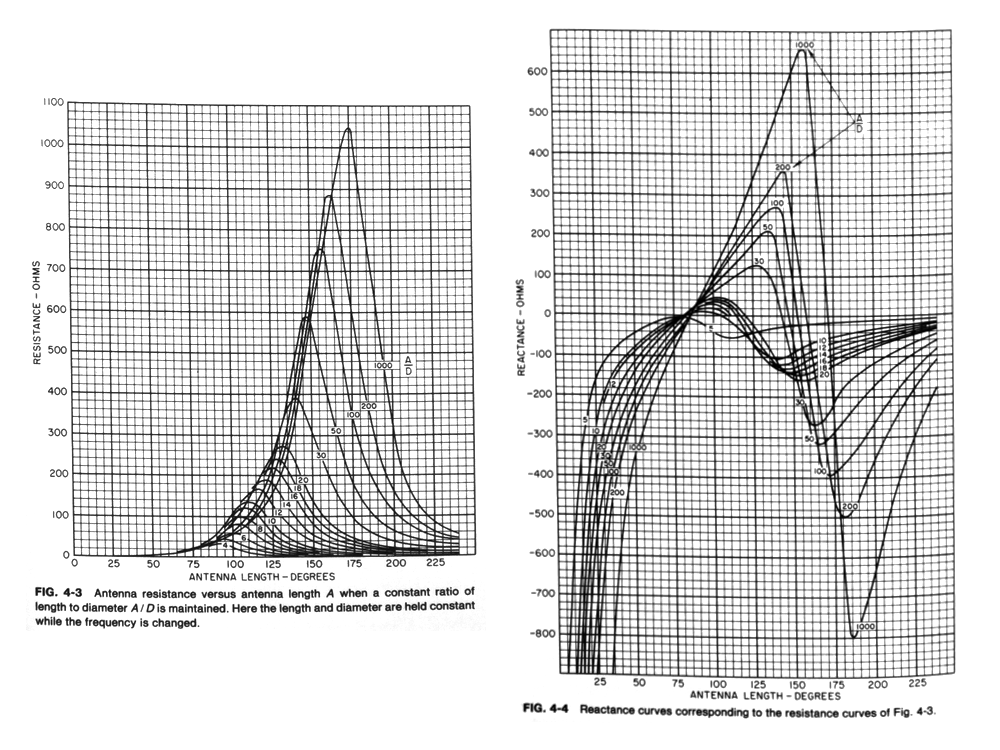
A half-wave dipole illuminating a parasitic array will often require a
"step-up" in feedpoint impedance to properly match the surge impedance
of popular transmission lines. Extending the physical length of a
monopole or dipole causes a slow rise in radiation resistance.
Contracting the length has the opposite effect. This phenomenon is
illustrated in the Brown-Woodward curves published in Chapter 4 of the
Antenna Engineering Handbook:
This often ignored property of monopole and dipole antennas makes it
possible to achieve a wide spectrum of feedpoint impedances suitable
for virtually any application.
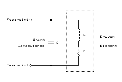
The only consequence of modifying the radiator's physical length beyond
the point where natural resonance occurs is that the feedpoint impedance
becomes highly reactive. In fact, the reactance varies more rapidly in
magnitude than does radiation resistance as the length of the radiator
is moved away from resonance.
The feedpoint impedance's reactive component is easily cancelled by
placing conjugate reactances in series with the feedpoint of the radiator.
When the added reactance is made equal in magnitude and opposite in
phase of that presented by the radiator, a pure resistive impedance
equal to that predicted by the Brown-Woodward curves is realized.
A shunt reactance can be placed in parallel with the feedpoint to
cancel the reactive component of the driven element's impedance as well.
However, what happens in the process is rather complex, and is not as
trivial as simply making the shunt reactance equal and opposite to that
of the driven element's reactance. Instead, a parallel resonant RLC
circuit is formed, and the radiation resistance seen at the feedpoint
is stepped up in the process to a level significantly higher than what
the Brown-Woodward curves alone predict.
Provided a step-up in feedpoint impedance is desired, a wide range of
impedances can be obtained simply by selecting the radiator's physical
length and shunt reactance appropriately. In fact, it almost doesn't
matter whether the driven element is adjusted to a physical length
above or below resonance. There's likely an impedance matching
solution for either situation.
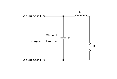
Shunt Capacitance Impedance
Matching Analysis
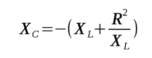
When a driven element exhibiting inductive reactance is brought to
resonance by introducing a capacitive reactance in parallel with the
element's feedpoint, the following equivalent RLC circuit is developed:
The shunt capacitive reactance, XC, required to resonate a
complex load exhibiting a pure resistance, R, in series with a distributed
inductive reactance, XL, can be computed as follows:
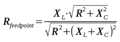
After applying the shunt capacitive reactance, XC, across the
driven element to bring the system into resonance, the resulting feedpoint
resistance, Rfeedpoint, can be computed as follows:
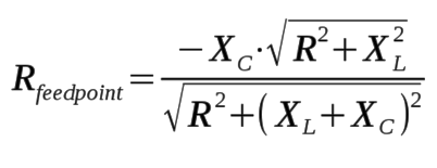
Note that all resistances and reactances are expressed in ohms, with
XC expressed as negative in magnitude.
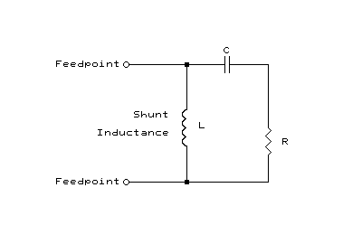
Shunt Inductance Impedance
Matching Analysis
A very similar impedance matching function, including a step-up in
feedpoint impedance, can be realized if a shunt inductance is connected
across the feedpoint of a driven element that is shorter than physical
half-wave resonance. Here is the equivalent RLC circuit:
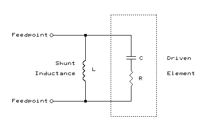
The shunt inductive reactance, XL, required to resonate a
complex load exhibiting a pure resistance, R, in series with capacitive
reactance, XC, can be computed as follows:

After applying the shunt inductance, XL, across the driven
element to bring the system into resonance, the resulting feedpoint
resistance, Rfeedpoint, can be computed as follows:
In other words, much like the shunt capacitance impedance matching
technique, a step-up in feedpoint impedance is realized by applying
a shunt inductance across a capacitive load, despite the reduction
in radiation resistance caused by decreasing the length of the radiating
element to produce the needed capacitive reactance.
Shunt inductance impedance matching is often employed in HF mobile antenna
installations when the radiating element is less than a quarter-wavelength
in height and an impedance step-up to match a 50 ohm transmission line is
desired. A "loading coil" of suitable inductance is connected
in series between the bottom of the radiating element and ground. If the
element length and the inductance of the coil are properly chosen, not
only is resonance established, but a 50 ohm feedpoint impedance across
the coil is also achieved.
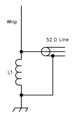
Shunt Inductance Impedance Matching for a Less Than One Quarter Wavelength Monopole
Another example of where shunt inductance impedance matching is employed is
in "Hairpin" Impedance Matching Networks.
Hairpin Impedance Matching
A "hairpin" is a shunt inductance placed across the feedpoint of a
capacitively reactive load to raise the resistive component of its
impedance. It is typically fabricated from parallel lengths of wire
forming a balanced transmission line that is less than 45 degrees in
length and shorted on the far end, making it purely inductive.
For many years, the ARRL Handbook published a design for a 5-element 50
MHz yagi that employed a "hairpin" across the antenna's dipole
driven element to raise its impedance to 200 ohms. Connection to a 50-ohm
unbalanced feed-line was made through a 4:1 half-wave coaxial balun.
The description of the antenna cautions the reader that the driven
element is the shortest element of the entire array. The article states,
"While this may seem a bit unusual, it is necessary with the hairpin
matching system".
Relationship To L-Network
Impedance Matching
The reason these impedance matching techniques produce an impedance
step-up in either configuration is because they are really L-networks with
their high-impedance, shunt reactance side positioned at the feedpoint,
and their low-impedance, series reactance side connected in series with
the driven element's radiation resistance:
Shunt Capacitance Equivalent Circuit
Shunt Inductance Equivalent Circuit
Another interesting relationship occurs with these networks. When the
network is properly adjusted to the point of resonance, the ratio of
radiation resistance to series reactance is always equal to the ratio
of shunt reactance to feedpoint resistance. Knowing this relationship
makes the calculation of feedpoint resistance significantly easier than
previously described once the shunt reactance is first determined.
Some Yagi Impedance Matching Examples
Using YAGIMAX 3.11 software, the feedpoint impedance of 18 element 432 MHz
DL6WU Yagi was estimated to be 34.23+j0.24 ohms using a 33.1978 cm long
driven element (dipole) at 432.200 MHz. Such a termination impedance
would produce a VSWR of appoximately 1.52:1 on a 52 ohm transmission line.
If the driven element is lengthed to 34.450 cm (below resonance), the
feedpoint impedance rises to 42.43+j20.06 ohms. Using the equations
illustrated above, when a capactive reactance of 109.8 ohms (3.35 pF)
is placed across the feedpoint of the driven element, a 51.9 ohm purely
resistive feedpoint impedance is obtained.
Going in the opposite direction, if the driven element is shortened to
31.6 cm (above resonance), a feedpoint impedance of 26.07-j25.95 ohms is
obtained. Using the equations illustrated above, when an inductive
reactance of 52.14 ohms (19.2 nH) is placed across the feedpoint of the
driven element, a 51.9 ohm purely resistive feedpoint impedance is
again obtained.
A balun is required to symmetrically feed a balanced driven element with
an unbalanced coaxial transmission line. 4:1 half-wave coaxial baluns
are often used, and require that the feedpoint of the Yagi be 200 ohms
in order to yield a 50 ohm output impedance.
If the driven element is lengthed to 39.57 cm, a feedpoint impedance of
102.03+j100.11 ohms is obtained. A shunt capactive reactance of 204.1 ohms
(1.8 pF) across the feedpoint yields a purely resistive impedance of
200.2 ohms. Note that under this tuning condition, the driven element
is physically 13% longer than the reflector, but is the proper
electrical length for the Yagi to function correctly.
Going in the opposite direction, if the driven element is shortened to
29.665 cm, the feedpoint impedance becomes 18.71-j58.30 ohms. A shunt
inductive reactance of 64.3 ohms (23.67 nH) yields a resistive feedpoint
impedance of 200.3 ohms. Under this tuning condition, the driven
element is shorter than the first four directors, but as before,
is the proper electrical length to function correctly.
Shunt Capacitance Impedance
Matching Network Calculator
The following Javascript calculator will determine a dipole's radiation
resistance once the resistive and inductive reactive components of the
dipole's feedpoint impedance are known, and the indicated shunt capacitance
is applied across the feedpoint terminals:
Shunt Inductance Impedance
Matching Network Calculator
The following Javascript calculator will determine a dipole's radiation
resistance once the resistive and capacitive reactive components of the
dipole's feedpoint impedance are known, and the indicated shunt inductance
is applied across the feedpoint terminals:
Conclusion
Whether the feedpoint impedance of a Yagi's driven element is raised using
a shunt capacitance and a slightly longer-than-naturally resonant driven
element length, or a shunt inductance and slightly shorter-than-naturally
resonant driven element length may be academic. In either case, the
step-up in feedpoint impedance occurs that is due primarily to
the impedance transformation nature of the network itself in the shunt
capacitance scenario, and entirely due to the impedance
transformation nature of the network in the shunt inductance
impedance matching scenario.
The shunt inductance method has the advantage of providing a DC (static
discharge) path across the radiator, while the shunt capacitance method
utilizes a radiator having a higher radiation resistance, which results
in a matching network having a lower 'Q' and a wider operating bandwidth.
