By Lyle Koehler, KØLR
Downconverter with FET input stage
12 volt version with varactor tuning
Crystal calculator spreadsheet
Multipath propagation observations
Introduction -- This article describes a "software" receiver that uses a simple, low cost hardware downconverter in conjunction with sound-card software such as DL4YHF's "Spectrum Lab" or I2PHD's "SDRadio", which act as a tunable DSP-IF system. Spectrum Lab is a powerful piece of software that can be used for receiving a variety of signal modes, including very slow CW (QRSS) that must be read from a "waterfall" type of spectrogram display rather than being copied by ear. SDRadio does not provide a built-in capability for QRSS, but is very convenient and easy to use for single sideband, CW, AM and ECSS (Exalted Carrier Selectable Sideband) reception. You can download Spectrum Lab from DL4YHF's Web site, and a beta version of SDRadio is available at I2PHD's software defined radio site. Because of its ease of use, SDRadio is a good choice for the initial checkout of the downconverter and your sound card system. Most of the references to sound card software in this article are to Spectrum Lab, but notes on the operation of SDRadio are included at the end of the article.
Note: Several references are made to other articles I have written, which can be found at my home page.
Most LowFER operation today utilizes weak-signal modes that require a computer to decode, or at least display, the signals. A few years ago, it required a trained ear and a receiver with very narrow filters to dig weak LowFER signals out of the noise. Now all of that work is done by the computer's sound card and digital signal processing (DSP) software. And that expensive box of receiving hardware sitting on your bench does little more than act as a frequency converter to translate signals in the LF (30 to 300 kHz) range down to a frequency that can be handled by the sound card in a computer. Typically the maximum sampling rate for a computer sound card is 48 kHz (although most applications will only show available rates up to 44.1 kHz), and the Nyquist limit says that the sound card can handle input signals up to half of that frequency, or 24 kHz. The popular "Argo" spectrogram software uses a lower sampling rate, and will accept incoming signals up to about 2.7 kHz.
Since the receiver is actually only serving as a down-converter, theoretically it can be replaced by a mixer and a local oscillator. In ham radio circles, that's known as a "direct conversion" receiver, and the direct conversion circuit is very popular for simple homebrew receivers. Some of them perform amazingly well for CW and SSB reception on the HF bands. There are a few disadvantages to direct conversion. One problem is that the receiver responds to signals on both sides of the local oscillator frequency, so you have to contend with twice the noise and interference that you'd get with a "single signal" receiver. There are ways to get rid of the image by using two mixers and phasing techniques, but now we're getting out of the "simple" receiver category. Another disadvantage is that the incoming RF signals may be in the microvolt level, and it requires volts or millivolts to drive headphones or a speaker. If you try to do all of the necessary amplification at audio frequencies, it takes really careful design to avoid hum pickup and oscillations. The so-called superheterodyne circuit avoids these problems by converting the signal to an intermediate frequency (IF), where much of the filtering and amplification takes place. Modern high-performance receivers typically use two or more conversion processes and intermediate frequencies. The first IF is chosen to be high enough so that the image frequency can be rejected easily by the front-end filters in the receiver. The final IF is low enough to make it easy to achieve the desired narrow bandwidth, or selectivity. Within the past few years, a number of receivers and ham transceivers have started using "IF DSP", where the final IF frequency is in the range of perhaps 30 to 40 kHz, and the filtering and demodulation functions are performed by digital signal processing software.
The LowFER receiver described in this article is a highly simplified version of an IF DSP receiver. At LF, it doesn't take a lot of front-end selectivity or a very high IF frequency to achieve usable (not necessarily good) image rejection. Suppose we choose an IF of 10 kHz, That puts the image frequency at 20 kHz away from the desired signal. If the response of the receiver's front end filter is down 10 or 20 dB and if there are no strong signals at the image frequency, the receiver might perform almost as well as a much more expensive commercial unit. In order to receive today's narrowband LowFER modes, we still need extremely good frequency stability and accuracy, and the ability to tune the receiver to the desired signal frequency. But if the tuning range isn't too wide, it can be done by tuning the IF rather than the local oscillator. For example, we can cover the 180 to 190 kHz range, where most US LowFERs operate, with a fixed local oscillator frequency and an IF that can be tuned over a 10 kHz range.
To put together a respectable LowFER receiver, I wanted a DSP IF that would tune from about 10 to 20 kHz, with a fairly narrow audio filter and a "comfortable" BFO pitch. Of course, the computer doesn't care what the pitch of the audio output signal is, but I like to listen to the few remaining CW beacons. I also want to hear what the receiver is picking up, even though the actual LowFER signal I'm trying to receive may be too slow to copy by ear, or buried 20 dB below the noise. Simultaneously, so that I don't have to pipe the audio output to another computer, I want to be able to display a spectrogram of the output signal, do automatic screen captures, save WAV files of the output, etc. That's a pretty big wish list. However, the "Spectrum Lab" software by DL4YHF can do all of those things. In fact it will do a lot more, once you learn how to use all of the features.
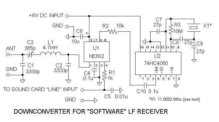
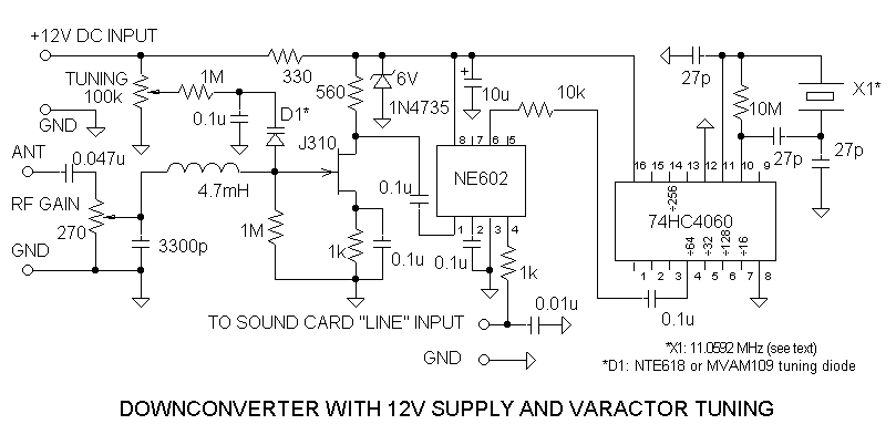
Designing the actual receiver hardware was easy. All I needed was a down-converter, so I borrowed most of the circuit from the LF up-converter described elsewhere on my web page in the "solderless homebrew projects" article. To cover the 180 to 190 kHz range, with a tunable IF of 10 to 20 kHz, the local oscillator frequency needs to be either 170 or 200 kHz. 200 kHz is a bad choice, because that would place the image frequency in the range where there are lots of strong non-directional beacons (NDBs). Crystals for the 170 kHz range are a bit hard to come by, but an HF crystal and a divider IC offer an easy and inexpensive solution. One of the common microprocessor crystal frequencies is 11.0592 MHz, which comes out to 172.8 kHz when divided by 64. I decided that this was close enough. The circuit of the down-converter, shown below, consists of an NE602 mixer (NE612 or SE612 parts are equivalent) and a 74HC4060 oscillator/divider operating in the divide-by-64 mode. Dan's Small Parts may have most of the parts required for this circuit. I didn't see the 11.0592 MHz crystal in his catalog, but he may have a 5.5296 crystal which only requires changing the output pin of the 74HC4060 from pin 4 to pin 5. To receive signals at 137 kHz, it is necessary to select a crystal so that the local oscillator is in the vicinity of 150 kHz. A "low side" local oscillator would not be a good idea because the image would be down in the really serious Loran splatter. Examples of acceptable crystals for 137 kHz reception are 10 MHz (divided by 64) or 4.9152 MHz (divided by 32). The exact frequency of the local oscillator is not critical, as long as it is stable, because the tuning is accomplished in the DSP IF. However, you do need a way to determine the crystal's frequency, and to calibrate the sound card's sampling rate if you are going to try for very slow modes like QRSS30. When looking for needles in a haystack, it really helps to know which haystack! Possible methods for calibration are discussed later in this article.
The receiver, like its up-converter predecessor, was built on a solderless protoboard. In the future I may revise the circuit to use varactor tuning with an MVAM109 or NTE618 diode in place of the air variable capacitor, and with a FET stage in front of the mixer to improve the gain and selectivity. But this is the circuit that was used for the "WE" and "WEB" reception examples described below. The receiver drew 8 milliamps when operated from my 6-volt regulated supply. It could also be run on 4 AA cells, or from a higher voltage supply with a dropping resistor to keep the voltage within the limits for the integrated circuits. For example; 9 volts with a 390 ohm resistor or 13.8 volts with a 1k resistor.

Assembled LF Downconverter
During the tests, the Spectrum Lab software ran on a 900 MHz Pentium III computer with 512 MB of RAM and a Creative Labs SoundBlaster Live sound card. Even though the DL4YHF software is well documented, I would have a hard time starting from scratch and getting it to do everything I wanted for this application. Fortunately the software comes with some pre-programmed examples that require only minor tweaking to get the desired result. I started with the "SAQ receiver" settings, which can be used to receive the 17.2 kHz transmissions from the historic longwave transmitter at Grimeton, Sweden when it is fired up once or twice a year. The default BFO pitch is 650 Hz, although I prefer something down around 450 Hz for receiving weak CW signals. With the local oscillator in the down-converter at 172.8 kHz, and an incoming signal at 185.3 kHz, the IF is at 12.5 kHz. Going into the Spectrum Lab's "components" window, I set the IF DSP local oscillator to 11850 Hz, which produced the required 650 Hz offset, and connected the receiver input to my pre-amplified loop. After peaking the tuning capacitor (there is a delay between the signal input and the audio output, so you have to tune very slowly), there was a good strong signal from LowFER "WE", who is about 70 miles from me. Later I changed the audio filter center frequency to 450 Hz and set the DSP local oscillator to 12050 Hz, which is where things were set to record this WAV file of WE's CW identifier. The original file as recorded by Spectrum Lab sounded cleaner, but I cropped and compressed the audio to reduce the file size.
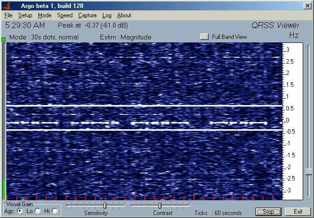
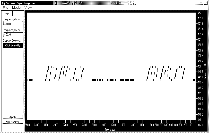
It took quite a bit of tweaking to set up the spectrogram feature of Spectrum Lab to receive the 1-watt, 189.950 kHz QRSS30 signal from Bill Bower's "WEB" beacon in Texas. When Bill was in Oklahoma, I could usually hear his OK beacon every night, but now it's a little more of a challenge. I will try to provide more details if I get to the point where I understand better what I'm doing, but the basic FFT settings were: Decimate by 16; FFT length 65536; 2000 millisecond scroll interval. The IF local oscillator was set for 16700 Hz (I'll leave the arithmetic up to the student), and I used a signal generator to make sure the converter's input circuit was peaked to 189.950 kHz. I couldn't find a setting that made WEB visible prior to going to bed, but usually the band opens up a couple of hours before sunrise. So I set up for screen captures every 20 minutes and hoped for the best. In the morning, the screen captures looked pretty bad -- too much sensitivity, so they were full of psychedelic "snow". However, one of the many impressive features of Spectrum Lab is the scrolling buffer, which lets you go back through the last couple of hours of data. That, plus the fact that when you adjust contrast, brightness, etc., it affects the past screen as well as the future! By scrolling back through the data and adjusting the contrast and brightness settings, I was able to produce some readable and very colorful renditions of the WEB identifier, but finally settled on the conservative color scheme shown below.
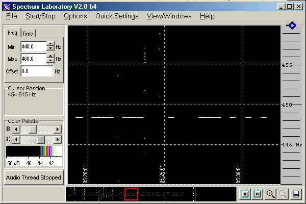
WEB beacon as received in Minnesota on November 9, 2003 (distance 1170 miles)
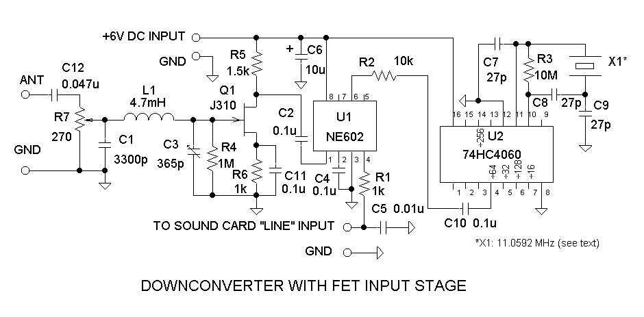
Downconverter with FET input stage -- After the first version of the downconverter seemed to be a success, I added a FET stage to the input, which provided some improvement in selectivity, because of less loading on the input tuned circuit, and a large increase in sensitivity. With this modification, the minimum detectable CW signal on the "software" receiver is well under 1 microvolt. The sensitivity is more than adequate for use with my passive single-turn 10-foot loop, or with a simplified version of the AMRAD active whip, without any additional preamplification. In fact, when I tried using my 8-foot tuned loop with the balanced high-gain preamp, the receiver overloaded. So I added an RF gain control potentiometer to the input circuit. The coupling capacitor C12 and gain pot R7 also help to prevent 60 Hz and DC signals from overloading the receiver or zapping the FET. Component values are not critical; for example a 1k pot will probably work just fine. I didn't include them in my circuit, but it might also be a good idea to add clamping diodes to protect the FET input. The diagram below shows the circuit of the "improved" downconverter. Adding the FET input stage increased the total current drain to approximately 10 mA. Note: While testing a later version of the converter, I found that the strong-signal handling capability of the FET stage improved considerably when R5 was reduced from 1.5k down to 560 ohms.
WE (70 miles) and NC (about 1030 miles) as received on a passive 10-foot loop
Now to the important subject of calibration. The software receiver's frequency accuracy is determined both by the crystal in the downconverter and by the sound card's sampling rate. I've always been pretty lucky with sound cards, but some people have observed errors of more than 1 per cent when displaying audio signals on a spectrogram. A 1 per cent error in an IF DSP local oscillator operating in the 10 to 20 kHz range would produce offsets of 10 to 20 Hz in the displayed spectrogram, which would typically be off scale when receiving QRSS or other narrowband modes. One of the great features of Spectrum Lab is that you can not only scroll back and forth in time, but also up and down in frequency. I have been using a filter bandwidth of 50 Hz, and I can scroll the spectrogram display +/-25 Hz before getting out of the filter bandwidth. However, when searching for weak signals it is very helpful to know exactly where to look, so the more accurate the receiver calibration, the better. The first step in the calibration process is to determine the accuracy of your sound card. Spectrum Lab lets you make corrections for sampling rate errors in the Audio Settings under the Options menu. But in order to do that, you need a precisely known audio frequency source. Fortunately, the crystal oscillator and the 74HC4060 divider can provide fairly accurate audio signals. I don't show the division ratios for all of the taps on the 74HC4060 in the schematic diagram, because there isn't enough room. But the available division ratios and the corresponding pin numbers on the 74HC4060 are as follows: 16 (pin 7); 32 (pin 5); 64 (pin 4); 128 (pin 6); 256 (pin 14); 512 (pin 13); 1024 (pin 15); 4096 (pin 1); 8192 (pin 2); and 16,348 (pin 3). Division ratios of 2, 4, 8 and 2048 are not available, and the direct output of the oscillator can be taken from pin 9.
With a crystal frequency of 11059.2 kHz, the divide by 1024 output of the 74HC4046 puts out a 10.8 kHz square wave. The frequency accuracy is only as good as the crystal -- if the crystal is off frequency by 100 parts per million, the error at 10.8 kHz is 1.08 Hz. But that's pretty good, if you don't have anything better available. To check the sound card, connect the output of pin 15 to the sound card's Line input through a large resistor. How big will depend on the input impedance of the sound card in your computer. I used a 10 meg resistor and still had a huge signal. Now open Spectrum Lab, go to the "Load Settings" option under the File menu, and select the file called SAQrcvr1.usr. This brings up a dual spectrogram display, showing the input to the sound card on the left, and the converted and filtered audio signal on the right. You will need to grab the frequency scale on the left-hand display and drag it with the mouse until the 10000 to 12000 frequency range is somewhere within the window. There should be a large peak in the spectrum at 10800. When you place the mouse cursor near the peak, a little green circle will jump to the top, and you can read the frequency from the "Cursor Position" box on the left. Bringing up the "Audio Settings" item under the Options menu will allow you to enter the correct frequency (10800) and the displayed frequency. Click on "calibrate"; then "apply", and now when you put the cursor on the peak it should read very close to 10800. You can make a further operational check of the DSP IF by going into the Spectrum Lab Components window (which probably opened automatically with the SAQrcvr1.usr file), and entering the number 10000 in the oscillator block. This will produce a beat note of 800 Hz, within the filter bandwidth, and you will probably hear a very strong 800 Hz tone in the speaker.
For more precise calibration of the sound card, you can try a similar procedure to view the horizontal oscillator frequency from a TV set. Connect an "antenna" (a long piece of wire will do) to the sound card's Line input, and bring it near a TV set that is receiving a stable picture. With luck, you will see a spike corresponding to the TV horizontal oscillator frequency. Here in the US, that frequency is supposed to be 15,734.26374 Hz and is usually very tightly controlled.
Calibration of the downconverter's local oscillator frequency is more difficult, unless you can find a clearly identifiable signal of known frequency. It's easiest if you have a very accurate signal generator in your shack, or a nearby LowFER with a big signal. But even if you don't, other signal sources are fairly widely available. One possibility is the 60 kHz signal from WWVB, which you can receive with an 11.0592 MHz crystal in the converter and a very minor circuit modification. The receiver front end won't tune down to 60 kHz with the components shown in the circuit diagram, but WWVB is so strong in many parts of the country that it may come through anyway, especially if you are using a broadband receiving antenna like the AMRAD active whip. The only modification really necessary for 60 kHz reception is to change the division ratio by taking the output from the divide by 256 tap (pin 14) on the 74HC4060. This results in a local oscillator signal of 11059.2/256 = 43.2 kHz. The IF output of the converter will be at 60 - 43.2 = 16.8 kHz, so look for that line in the SAQrcvr1 left-hand spectrum display. To verify that you are actually hearing WWVB, set the DSP IF oscillator frequency to 16000, and listen for the 800 Hz signal in the output. For those who have never heard WWVB, there are no voice announcements, only a slow time code that is sent by shifting the signal amplitude by 10 dB. It sounds like someone with a sloppy "fist" sending slow Morse code. What if the display shows something other than 16,800 Hz; for example 16,805 Hz? One solution is to work backwards and figure out what your crystal frequency actually is. In this example, since the WWVB signal appears to be 5 Hz high, it means that the downconverter's local oscillator is 5 Hz low, at 43.195 kHz. So the actual crystal frequency is 43.195 x 256 = 11.05792 MHz. Once you have this frequency, you can use it in your calculations to decide where to set the DSP IF oscillator, or how far to offset the spectrogram display. After all, this is supposed to be a "software" receiver. For hardware types who prefer to put the oscillator exactly on frequency, it can probably be done by replacing C9 with an 8-50 pF trimmer. However, there is no guarantee that a cheap microprocessor crystal will oscillate precisely on its specified frequency in this circuit.
Another possible calibration source is, again, the TV horizontal oscillator. The 12th harmonic falls on 188.81116 kHz, and with an antenna near the TV set, there should be a bunch of junk near that frequency with one larger spike in the center. Normally the TV oscillator harmonics are nothing but a horrible noise source on LF, and even on the lower HF bands, but perhaps they can be of some use after all.
Compared to the calibration process, actual operation of the receiver is relatively easy. Fortunately for me, my sound card and crystal were close enough so that I was able to try receiving first, and then worry about calibration later. Spectrum Lab has so many features that it takes a while to learn how to use it, and I'm still near the beginning of the learning curve. As mentioned earlier, it is very helpful to use a pre-programmed application as a starting point. If you download this user file: 185r3.usr and store it in the Spectrum Lab working directory (which already contains other files with a .usr extension), you should be able to load the settings from the "File" menu while running the program. Theoretically this will invoke all of the settings that I used to hear and capture 185.3 kHz signals with a downconverter that has an 11.0592 MHz crystal. The BFO pitch will be 450 Hz, with a 50 Hz filter bandwidth, and the spectrum display is also centered on 450 Hz with a -450 offset (450 Hz appears as zero on the screen).
To receive other signal frequencies or to use different local oscillator/divider combinations in the downconverter without changing any other parameters, it should only be necessary to open the Spectrum Lab "components" window, and type a new frequency into the local oscillator block. Suppose, for example, that you wish to receive WEB on 189.950 kHz, and that you are using a 1.70000 MHz source and a divide by 10 circuit to produce a 170 kHz local oscillator signal for the downconverter. An example of such a circuit can be found in the LF transmitter diagram in my solderless homebrew projects article. The IF signal will appear at 189.950 -170.000 = 19.95 kHz. To produce a 450 Hz beat note and to keep the spectrum display "right side up", the DSP local oscillator needs to be at 19.95 - 0.45 = 19.50 kHz. So you would enter the number 19500 in the oscillator block of the Spectrum Lab components window.
Here is another example, showing how to receive signals in the 137 kHz region: I wanted to look for Part 5 beacon "XFX" on approximately 137.781 kHz. With a crystal frequency of 10 MHz and a division ratio of 64, the downconverter's local oscillator signal is at 156.25 kHz, and the IF output is at 137.781 - 156.25 = -18.469 kHz. The negative number for the IF frequency means that the spectrogram display will be inverted; that is, as the incoming signal goes up in frequency, the trace on the spectrogram moves down. I figured that this could be corrected by using "high side" injection for the IF DSP local oscillator, setting it 450 Hz above rather than 450 Hz below the IF signal. Indeed, that seemed to work. The output of my signal generator appeared at just the right place on the spectrogram display, and when I peaked the input capacitor on the downconverter, I could hear the signal with the generator output turned almost as low as it would go, well below 1 microvolt. By the way, I had lucked out again with the cheap 10 MHz crystal -- the local oscillator frequency was within 1 Hz of where it was supposed to be. Unfortunately, when I connected the downconverter to my multiturn, tuned loop antenna, there was no trace of XFX, and the Loran lines were not in the right place. Another computer in the shack was running Argo to view the output of my IC-756PRO, which was connected to the same antenna and also tuned to 137.781. According to John Andrews' alliterative listing of Loran lines, there should have been only two strong lines from the Baudette, MN Loran transmitter, spaced about 1 Hz apart, with XFX someplace between them. That's what showed up on the Argo display, but Spectrum Lab displayed several lines, none of them with the proper spacing. Finally, in desperation, I set the DSP IF local oscillator frequency 450 Hz below the IF. Now the correct two lines and XFX showed in the display, and after going into the Spectrum Lab Options to invert the display, the spectrogram was right side up. I eventually found out why it was necessary to put the local oscillator below the IF signal -- Spectrum Lab lets you choose whether the mixer is an upconverter, downconverter, USB, LSB, DSB, etc. If I had selected "LSB downconverter", it probably would have worked the first time... The settings used for the XFX capture are available here as 137r781.usr.
My simple single-turn loop has a fixed capacitor that tunes it to approximately 185 kHz, and the response is too far down to produce a usable signal in the 137 khz range. I was also unable to see XFX with my "poor man's" version of the AMRAD active whip antenna feeding the downconverter. There is a good possibility that the downconverter is being overloaded by out-of-band signals, since the active whip responds to everything from VLF through HF. I have also noticed that when I connect the active whip to my HP3586B selective level meter, I often get an "overload" LED indication even though the amplitude meter is not off scale. Someday I'll try a preselector on the output of the active whip to see if that fixes the problem. In the meantime, the tuned multiturn loop with its high-gain preamp works well into the software receiver, although it was necessary to crank the input gain pot on the downconverter almost all the way to zero. The screen captures below cover the same time frame, and show how the software receiver and Spectrum Lab compare to my IC-756PRO and Argo, using the same input signal. It looks like the software receiver was doing a better job than the "big rig", but if the Argo settings had been just right, I am sure that it would have produced as "clean" a screen capture as Spectrum Lab. The nice thing about Spectrum Lab's scrolling buffer is that I was able to travel back in time, so to speak, and fix the settings. Like a "morning after" birth control pill!
XFX as received on an Icom IC-756PRO
XFX on the sofware receiver
This receiver has not been tested in an urban location with high levels of RF signals, so there are no guarantees on performance in that kind of situation. The screen captures shown in the early portions of this article were taken with the solderless protoboard version of the downconverter sitting on the workbench without an enclosure. No isolation transformers were used between the downconverter and the antenna or computer, except for the transformer that is part of the single-turn receiving loop. I was not aware of interference from my computers themselves, or from the dual monitors on my 900 MHz computer, which were about 6 feet from the downconverter. No doubt there were some strong interfering signals from the computers but they didn't happen to be on the frequencies I was watching. However, the monitor on my "ham" computer, sitting less than two feet away on the same workbench as the downconverter, pretty much wiped out reception of weak signals. I had to leave that monitor turned off during the overnight captures. Probably a shielded enclosure would help, because the 4.7 mH inductor in the downconverter acts as a miniature ferrite rod antenna.
Frequency stability of the prototype receiver was very good, considering that it had no enclosure and that it uses inexpensive microprocessor crystals. I did notice some drift when the electric heater was turned on in the shack. A PTC thermistor, soldered or epoxied to the crystal can as described in my "All in one" transmitter article, would probably improve the stability considerably, and for 137 kHz reception it would be easy to substitute a 10 MHz TCXO for the crystal.
12 volt version with varactor tuning -- The largest and most expensive component in the downconverter is the tuning capacitor. Maybe I shouldn't call it a "tuning" control, because it only peaks the amplitude response of the input circuit -- the actual frequency tuning is done in the DSP IF software. Anyway, when I finally transferred the circuit to a solder-type protoboard (Radio Shack number 276-150) and put it into a small enclosure (Digi-Key number L102), I used an NTE618 tuning diode in place of the air variable capacitor. With a 4.7 mH inductor in the circuit, the input response peak can be tuned from about 90 to 350 kHz. At the time of this writing, Mouser Electronics shows the NTE618 (part number 526-NTE618) in the on-line catalog, even though it may not be in the printed version. An MVAM109 from Dan's Small Parts should work equally well. I also added a dropping resistor and a Zener diode so that the circuit can be operated from a 12 volt supply. The current drain is about 20 mA. A circuit diagram of the varactor-tuned converter and a picture of the circuit mounted in the enclosure are shown below.
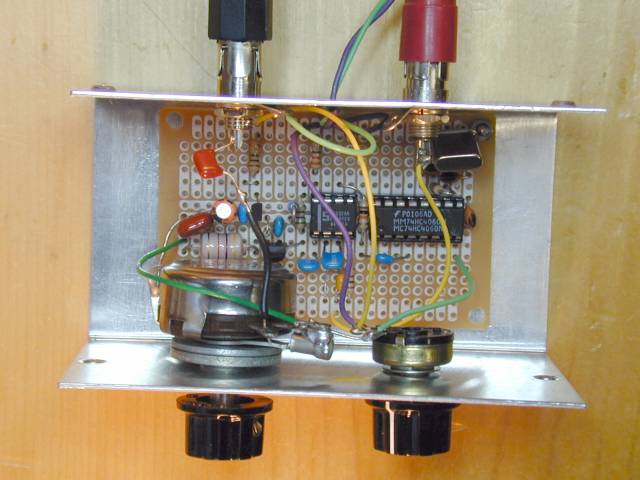
Varactor-Tuned Downconverter in 2.25 X 2.25 X 4 Inch Enclosure
Dual-Watch operation -- Spectrum Lab is capable of stereo processing, so that by feeding the left and right channels from a single downconverter (or from separate downconverters if desired), two frequencies can be monitored simultaneously. It is necessary to enable stereo processing under the "audio" settings in Spectrum Lab's Options menu, and also to enable the right-channel mixer, oscillator and amplifier. If the crossover amplifiers between left and right channels show up as active in the components display, they can be turned off by setting both gains to zero. The figure below shows what the "Components" window looks like when Spectrum Lab is set up to receive 185.3 kHz on the left channel and 182.2 kHz on the right channel, using an 11.0592 MHz (nominal) crystal in the downconverter. The audio filters are set for a center frequency of 450 Hz, and the local oscillator frequencies are offset by 5 Hz to compensate for the error in the crystal frequency. You can download the dual-w.usr file to provide a starting point for the "dual watch" settings.
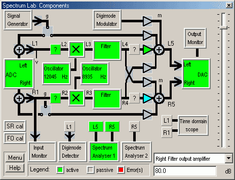
Components window showing settings for dual-watch operation
I found two minor quirks when trying to use Spectrum Analyzer 1 to display both channels on a split display. Strong signals in one channel bleed over into the other channel in the spectrogram, although they do not seem to be present in the speaker output. An easy fix would be to choose separate audio filter passbands for each channel. That's where the second quirk showed up. When I set up one channel for a center frequency of 450 Hz and the other channel for a center frequency of 500 Hz, it appeared that both channels were centered at 475 Hz. I haven't tried wider separations to see if that changes anything. For the present, I simply left both passbands centered at 450 Hz, but offset the spectrogram display (and the corresponding local oscillator) to center the right channel at 460 Hz while the left channel remained at 450 Hz. That at least keeps "WEOH" from showing up as a ghost above "BRO" in the sample screenshot below.
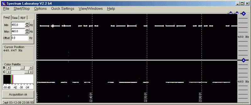
Spectrum Lab in "dual watch" mode, monitoring 185.3 and 182.2 kHz
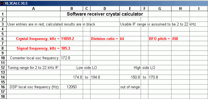
Crystal calculator spreadsheet -- A spreadsheet calculation is helpful for figuring out the local oscillator settings in Spectrum Lab, and for deciding which crystals in your junkbox might be usable in the downconverter. Here is a screenshot of a spreadsheet that I set up to do the routine arithmetic. I have also included a downloadable copy of the spreadsheet, called XL3CALC.XLS, which has been saved in Excel 3 format and which should work with later Excel versions as well.
For those who like to experiment, and who are able to adapt pieces of other circuits to new applications, it is possible to build a "frequency agile" downconverter with no crystals at all. My web page has an article, written a few years ago, describing how to build a phase locked loop (PLL) frequency synthesizer using the sound output of a PC as a reference signal. In that article, it was necessary to get into the PC and tap into the speaker leads to extract the audio signal. With Spectrum Lab and a duplex sound card, you can invoke a signal generator function that puts out a reference signal from the left channel of the sound card, while using the right channel as the DSP-IF system. I tried a quick breadboard using the same CD4046 PLL circuit that is shown in my PC-based synthesizer article, with a 4017 divide-by-10 circuit in the loop. When the Spectrum Lab signal generator is set to 17,000 Hz, for example, the PLL output is at 10 times that frequency, or 170 kHz. Other divider chips can be used, and the PLL circuit components can be varied to cover different frequency ranges such as the NDB band from 190 to 550 kHz. Although I didn't measure the frequency stability, which should be as good (or as bad) as the stability of the reference oscillator in the sound card, the frequency-agile downconverter worked well for copying LowFER CW signals and NDBs by ear. One problem I discovered is that the signal generator feeds into the right channel, even though the "switch" in the Spectrum Lab components window is set to direct the output to the left channel only. An acceptable workaround is to reduce the output of Spectrum Lab's signal generator to a very low level like -90 dB or less, and then increase the gain of the left channel amplifier by a similar amount to restore the signal to a usable level for the PLL circuit. This reduces the "birdie" produced by the signal generator to a very low level.
Notes on using SDRadio -- SDRadio is designed to provide an IF tuning range of +/- 24 kHz, giving a total tuning range of 48 kHz with a standard computer sound card that samples at 48 kHz. Seems like black magic, right? To take advantage of the full tuning range and to suppress the unwanted "sideband", you need a dual downconverter with quadrature local oscillators, and a sound card that does not introduce any appreciable delay between the left and right channel inputs. More information is available on the soft_radio discussion group referenced on the SDRadio site, and there are many other resources on the Internet if you search for "software defined radio". When used with the simple downconverter circuits described in this article, all of the features of SDRadio are available except that the tuning range is limited to 24 kHz, and image frequency suppression is only as good as the selectivity of the downconverter's input circuit. Available detection modes are AM, SSB and ECSS (Exalted Carrier Selectable Sideband), and the variable bandwidth feature is excellent for CW reception in SSB mode. FM detection may be a future option. Audio bandwidth, center frequency, etc are controlled with the mouse, and there is a real-time spectrum scope showing the relative amplitudes of all signals within the IF tuning range. The software is very intuitive and user friendly, but since it is still in beta test version, there are no published instructions or help files. Here are some brief notes that Alberto has provided to help explain the features:
SDRadio theoretically expects a couple of I/Q signals fed to the stereo input of the sound card. If you just have a single signal, it doesn't matter, send it to both left and right channels.The net effect will be that you will have not 48 kHz of spectrum available for software tuning with the mouse, but just 24, with the lower half mirrored in the upper half.
The blue window indicating the passband has both the borders draggable with the mouse. The window itself can be dragged in toto, selecting it in the middle. Anyway the cursor on the screen will dynamically change shape, indicating which operation you are about to do.
More fun with Spectrum Lab -- SpecLab is like the Swiss Army knife of sound-card programs. However, it can be awkward, if not downright dangerous, to use more than one tool on a Swiss Army knife at the same time. With SpecLab there is no problem using a bunch of functions at once, unless your computer runs out of processing and memory resources. The following set of examples was obtained on a Pentium 900 processor with 512 MB of RAM running Windows ME. While SpecLab was doing all of these things, I was also sending and receiving e-mails with Outlook Express, looking at Web pages with Internet Explorer, and capturing the screen and converting images in IrfanView. No doubt the computer was running low on resources, but it didn't freeze up or display the blue screen of death. Although the images below were not all obtained at the same time, the functions they represent were all running simultaneously in SpecLab. The filtered audio output from one selected center frequency (in this case, BRO's frequency of 182.2 kHz) was available from the computer speakers at the same time. I could have used SpecLab to capture a .wav file, too.
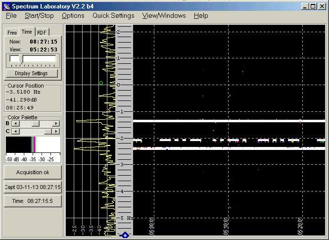
The basic display in SpecLab is of "Spectrogram 1". You have a choice of waterfall type display, spectrum display, or both, in horizontal or vertical format. I chose the vertical waterfall for this example because I was watching a fairly wide piece of the LowFER band; from about 181 kHz to just above 190 kHz. The receiving antenna was the single-turn passive 10-foot loop, oriented N-S, with a 20 dB preamp in front of the downconverter. A preamp is not needed when the downconverter's tuning control is peaked at a single desired signal frequency, but in this case I was trying to "flatten" the response across a 9-kHz bandwidth. The loop has a fixed series capacitor that peaks its response somewhere below 185 kHz, and the varactor tuning on the downconverter was adjusted to bring up the upper portion of the band. This gives a frequency response that is far from flat, but good enough so that the three frequency ranges of interest -- 182.2, 185.3 and 189.95 kHz -- are all within the dynamic range of the waterfall display. My downconverter local oscillator was at 172.8 kHz, so an input frequency range of 181.0 to 190.0 kHz corresponds to an IF range of 8.2 to 17.2 kHz. I offset the frequency scale by 7.2 kHz so that 5.00 kHz on the scale corresponds to 185.00 kHz, etc. The color palette I selected was all greyscale, except for the "current" trace in the spectrum plot. I'm not sure why the current trace at that moment is so much higher than the average value. It's easy to explain the hashmarks that appear for about two minutes starting at 0700, though. The lamp next to my bed is controlled by wireless switches and an X10 lamp module. During the two minutes it took me to get dressed, the good old light-dimmer noise totally wiped out the band even though the antenna is isolated and about 150 feet from the house. This screenshot also shows the multitude of very strong power-line carriers and other garbage signals that are always present on the LowFER band at my location.
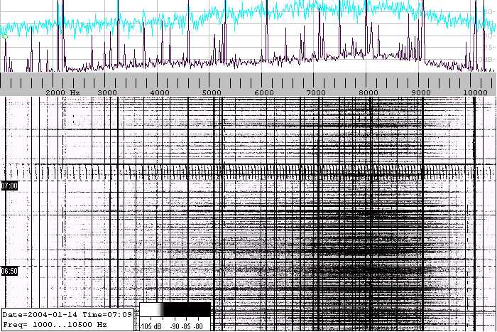
Spectrum Lab display of 181.0 to 190.5 kHz (Spectrogram 1)
If you look carefully, you can see "RO" near the bottom of the waterfall display at 2.20 kHz, before BRO goes into MT-Hell mode and produces what look like strange "Morse" characters on this low-resolution display. WEOH is visible at 5.30 kHz but none of the other members of the watering hole gang were strong enough to be seen. At 9.95 kHz, there is a "B" and then a "WE", ending just before WEB was scheduled to go into 6 WPM CW mode at 0700 CST. Actually WEB was stronger a half hour earlier, but I had not set up SpecLab for automatic screen captures because I didn't really expect to see anything but the local LowFERs on this wideband display. So the only screenshot I have is this manual capture, taken a few minutes after 0700 CST. The scrollback buffer in SpecLab is a great feature, but with the FFT and memory settings I was using, the buffered display is only about 1.3 kHz wide. If I had tried to scroll back in time, or even tried an after-the-fact adjustment of the display settings, all of the data outside that 1.3 kHz bandwidth would have disappeared from the screen except for approximately the last 20 minutes. That is not normally a limitation, unless you are trying to go back and view a large range of frequencies on each side of center.
Earlier in this article I showed an example of a signal displayed on the second spectrogram. The screenshot below shows what BRO's signal looks like when I "zoom in" on it. Different FFT settings can be used for Spectrogram 1 and Spectrogram 2. For the broadband display in Spectrogram 1, which was taken prior to any mixing or filtering actions, I used an "FFT input size" of 65536 with a decimation factor of 1 and a sampling rate of 44.1 kHz. This gives a resolution of about 0.67 Hz. Spectrogram 2 was taken at a point in the "block diagram" where BRO's signal had been converted down to the 450 Hz range, and passed through a 50 Hz bandwidth filter and an amplification stage (all functions performed by the SpecLab software). Because the sampling rate divided by the decimation factor must be at least twice the input signal frequency, I couldn't apply any decimation to the broadband spectrogram, and 0.67 Hz was as narrow as it would go. For the second spectrogram, however, the FFT settings were: FFT length = 65,536; decimation factor = 16; bandwidth = 0.042 Hz. Theoretically I could have gone to a decimation factor of 32 but didn't want to strain the computer's resources any further. The resulting plot produces an interesting effect on BRO's MT-Hell characters.
Spectrogram 2 centered near 182.2 kHz
One other very useful tool in SpecLab is the "Watch List and Plotter" function. You can monitor up to 20 different "channels" and plot selected parameters for each channel -- for example, the amplitude and/or frequency of the strongest signal within a specified frequency range. In the screenshot below I was monitoring the amplitudes of the strongest signals within 10-Hz bandwidths centered at 182.20 kHz (BRO), 185.30 kHz (WEOH), and 189.95 kHz (WEB). Actually I was also "watching" 189.80 for RM, but Roger's signal was off the air so I suppressed the display of that plot. The filter bandwidth for the plot function is defined by the Spectrogram 1 FFT settings, which in this case produced a bandwidth of 0.67 Hz. There is no automatic screen capture function for either Spectrogram 2 or the Plotter window, but there is a plot file buffer that lets you scroll back in time by an amount determined by the memory settings and how many channels are being plotted. With three channels and a memory setting of 10,000 samples, it is possible to scroll back over a time period of several hours. If you want to change display characteristics of the plot, such as amplitude range, pen color, etc., it can be done after the fact and will apply to the entire time history in the plot buffer. Plot files can also be exported to a text file and re-imported later for review.
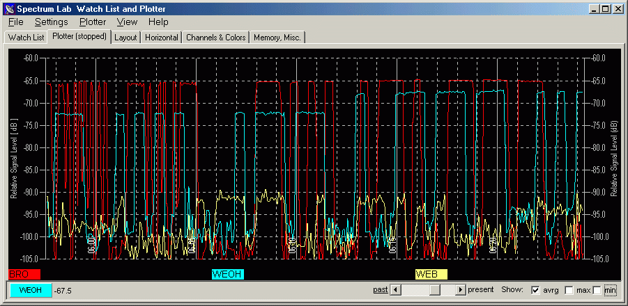
Signal level plots for BRO, WEOH and WEB
I selected this timeframe from the plot buffer because it shows two interesting things. First, it shows that a hardy Minnesotan like Mike will go out in the cold and dark at a little after 6 in the morning to switch from his omnidirectional flat top antenna to his N-S loop. Second, WEB's signal from 1170 miles away briefly reaches a level within 20 dB of Mike's flat top. Obviously the skywave propagation was really good for the period from about 0605 to 0618 CST on January 14th, 2004.
Multipath propagation observations -- A plot of signal strength versus time offers a much better picture of what the propagation path is doing than the typical waterfall type of spectrogram display. Until recently, I was of the belief that skywave effects were of little significance for stations within 100 miles because at low frequencies, the ionosphere is not supposed to be a very good reflector for high angle signals, so the surface-wave component should always dominate. However, reception reports from Bill Ashlock's crossed transmitting loops indicated that skywave effects were present even at fairly short distances. The real clincher came when Mike and Bill installed an east-west loop for Mike's "WEOH" beacon, which is about 70 miles away and nearly straight south of me. I expected to see a significant reduction in signal strength when compared to either Mike's north-south loop or his top-loaded vertical. But while watching the WEOH plot on the first evening of operation on the E-W loop, the signal strength was literally all over the map; sometimes dropping almost into the noise at my location and then bouncing back up again. At the same time, WEOH was showing up very well on the "Grabulator" (live Argo captures) provided by Steve, W3EEE in Pennsylvania. Obviously thre was nothing wrong with Mike's radiated signal, so propagation had to be the culprit even though we are within easy surface-wave range.
In the past, I've seen very small diurnal fluctuations in the signal strengths of local LowFERs as observed on the receiver S meter, but the effect was slight and could be attributed to other factors such as day-night temperature variations that might affect the radiation efficiency of the vertical antennas we were all using. But I never tried plotting anyone's signal strength, and probably would not have seen much variation anyway. That's because we were using verticals, which are omnidirectional so you can't be in a pattern null, and they don't radiate well at the very high elevation angles that would be associated with short-range skywave propagation. Now Mike comes along with an E-W loop; I'm near the broadside null (at low angles) in his pattern; and loops in the vertical plane radiate just as well straight up as they do at low angles. That changes everything!
Here is a plot of the amplitudes of LowFERs BRO, WEOH and RM, starting at about an hour after sunrise on January 15th, 2004. The gain of the receiver varied considerably at the different frequencies of these signals, as shown in the earlier spectrogram covering 181 to 190 kHz. You can't determine from the peak amplitudes how much stronger BRO is than RM, for example. Looking at the signal to noise ratio might be slightly more accurate, but even then the noise could be different at different frequencies. So the main purpose of this plot is to establish a "daytime" baseline for the signal levels from each individual beacon. By this time of day, skywave propagation on LF usually shuts down, although anything can happen in Winter (perhaps even in Summer)! Since everybody's signal strength is nearly constant over a half-hour period, it looks as though no strange propagation is taking place and we are probably looking at the surface wave signal. My receiving loop was oriented N-S, which favors WEOH, but BRO and RM are not in a pattern null.
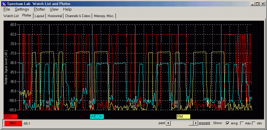
Daytime plot of BRO, WEOH and RM signal strengths
Now let's go back and see what was happening before sunrise. Actually WEOH's signal may have been fluctuating even more wildly during the previous evening, but this plot is interesting because everybody's doing it! The variations are not as great on BRO's and RM's signals, but they are definitely not as stable as in the daytime. Some fluctuation can be the result of higher noise levels at night. However, there seems to be a very distinct fade cycle on BRO, and RM shows a similar pattern. Both of those stations are northeast of me in the Duluth, MN vicinity and are about the same distance from me (70 miles) as WEOH.
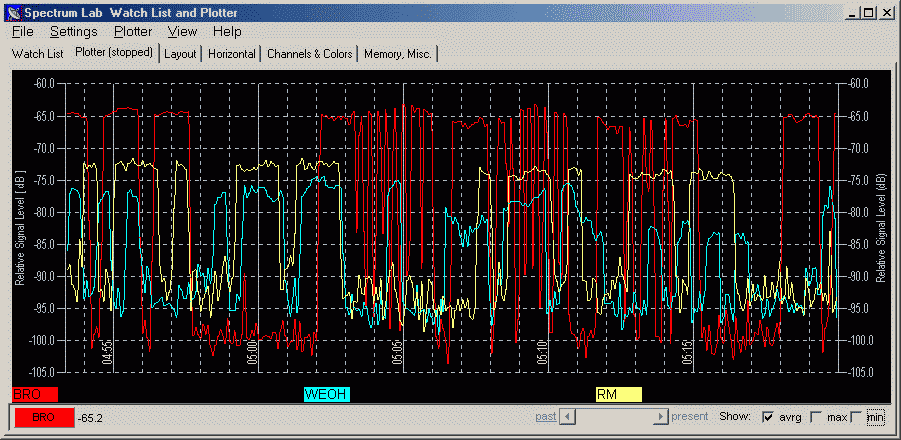
Night-time plot of BRO, WEOH and RM signal strengths
Now I'll try to explain why Mike's signal is affected so much more than Bryce's and Roger's, and will also attempt to put some numbers on the skywave signal contribution. This is dangerous because I'm not a propagation expert by any means, but at the same time I don't have any professional reputation to worry about, so here goes.
If two signals are combined, and one is much smaller than the other, the difference between "constructive interference" (signals adding) and "destructive interference" (signals subtracting) is very small. But when two signals that have travelled over different paths have exactly the same amplitude, the total signal strength will be doubled (+6 dB) at the peak of constructive interference, and the strength can go all the way down to zero during destructive interference. Looking at BRO's signal, I see perhaps a +/-2 dB variation in strength during a fade cycle. That says that the field strength is varying by about +/-26 per cent. Taking 20*LOG(.26), I get -11.7 dB. The skywave signal is down only 11.7 dB? I would have guessed at a much lower number! OK, let's look at the earlier Signal level plots for BRO, WEOH and WEB, which were taken when WEOH switched over from the top-loaded vertical to the N-S loop. Although the time was more than an hour before sunrise, both WEOH and BRO were very stable, and Mike's signal level was about -67.5 dB on the N-S loop. Comparing that with the daytime plot, WEOH's signal on the E-W loop is about -80.5 dB, roughly 13 dB lower than it was on the N-S loop. But both loops probably radiate about the same amount of signal at very high elevation angles. There are polarization issues, but if LF skywave propagation is anything like HF (which may or may not be true), polarization gets all messed up in skywave propagation anyway. So it's entirely plausible, that WEOH's signal could increase by 6 dB (or more, if skywave attenuation is really low) during the peak of a fade cycle, and drop into the noise level during minima. In fact, we see the WEOH signal reaching a level of about -75 dB at one point during the night-time plot, which is almost 6 dB higher than the daytime signal. Interesting...