Automatic In-phase Quadrature Balancing AIQB

Oscar Steila, IK1XPV , October 2006 (Rev C: 7/10/2012) www.qsl.net\ik1xpv

Many Hams started to play with digital signal processing and direct conversion receiver on a PC [5][7] or on dedicated processors[6] , following the technology appeal of Software Defined Radio solution. Different imbalance compensation schemes have been implemented [1]-[4].

In this paper a blind imbalance correction technique is described. This algorithm has been implemented in CIAOradio digital signal processing program [12].

One of the limiting issue in direct down-conversion receiver or low frequency IF receiver is I/Q imbalance and the resulting low image frequency cancellation. The imbalance is attributed to the mismatched components in the in-phase (I) and the quadrature (Q) branches.

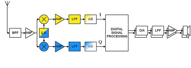
Fig 1- Direct down-conversion receiver

Problem rises from imperfectly balanced local oscillator (LO) and/or base band low pass filters (LPF) with mismatched frequency responses. An ideal down-converter performs simple frequency shifting. A down-converter with I/Q imbalance not only down-converts the desired signal, but also introduces its image interference

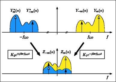
Fig.2 - Direct-conversion with I/Q imbalance

Direct-conversion with I/Q imbalance can be interpreted as a superposition of a desired complex down-conversion and an undesired complex up-conversion.

Although the I/Q imbalance introduced by the LO may be assumed constant over the signal bandwidth, the mismatches in the subsequent baseband I/Q amplifiers and filters vary with frequencies.

Frequency dependent I/Q imbalance is particularly severe in a wideband direct-conversion receiver and the corresponding estimation and compensation process becomes more challenging [2].

Abundant literatures exist on I/Q imbalance compensation see [1]–[4] and references therein.

In this paper we assume the signals are sampled and satisfy the sampling theorems and we focus on low pass component of modulation signals referred to Radio Frequency (RF) carrier.

The most immediate way is to correct the imbalance is a trigonometric approach to compensate it with a sample rotation and amplitude adjust.

x_i = x_i

x_q = x_q• a + x_i • b

where:

a = g ⁄ cosθ

b = g •tanθ

g = gain correction

( ideally 1 )

θ = phase correction

( ideally 0°)

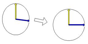
Fig.3 - Sample rotation and amplitude adjust.

The procedure can be implemented using two multiplication and a single addition every sample [1].

The gain and phase parameters must be adjusted to get the best performance.

The scheme is not able to compensate phase and gain distortions that vary on frequency.

Assuming to have a wide band signal in the desired part of spectrum, the image compensation will get the best result only in a part of the image spectrum.

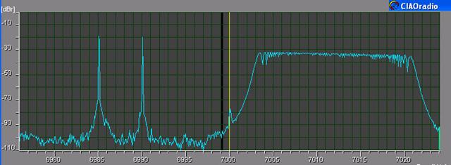
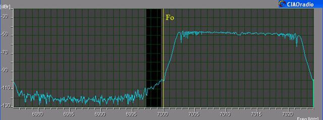
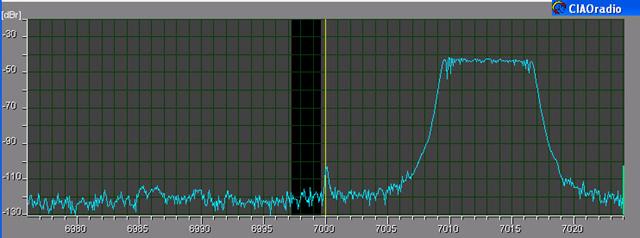
Fig.4 – CIAOradio reception of a test signal with 7002-7022 kHz spectrum

The picture is taken from CIAOradio program screen. It shows the receiver spectrum around Fo, with manual adjust of rotation and amplitude only. Notice that the image rejection depends on frequency.

An approach the frequency dependent linear imbalance compensation rises from the use of a compensation filter that equalize the I and Q channel response.

In CIAOradio design the filtering and tuning are done using the fast convolution.

A Digital Fourier Transform of input is made via a complex FFT. This dsp block analyze the frequency spectrum with a resolution in the order of 12Hz (48kHz sampling/4096 point FFT).

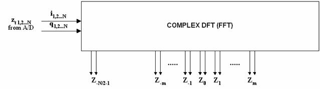
Fig.5 –DFT generates complex frequency sample

Every output bin of FFT carries phase and amplitude information of every frequency from –Fs/2 to +Fs/2 with Fs = sampling frequency (typ 48Khz).

The frequency selective imbalance will affect symmetric bins (to frequency 0), ie Z_m versus Z_-m ,

in different way, at changing of index m.

In [2] it is introduced a model in which the imbalance can be seen as the result of the imperfections a complex Local Oscillator (LO) signal with the time function:

ŝ_LO(t) = cos(2πf_LOt ) - jg sin(2πf_LOt + θ) (1)

where g is the amplitude imbalance, and θ indicates the phase balance.

We define the complex I/Q imbalance parameters as:

1 + ge^-jθ 1 - ge^+jθ

K₁ = ────── , K₂ = ────── (2)

2 2

In order to define the (1) as:

ŝ_LO(t) = K₁e^-j²^πf^LO^t+ K₂ e^+j²^πf^LO^t (3)

Direct-conversion with I/Q imbalance can be interpreted as a superposition of a desired complex down-conversion (weighted by K₁) and an undesired complex up-conversion (weighted by K₂).

Consequently, the received base band signal with I/Q imbalance z(t) is a superposition of the desired frequency band y(t) and its image y*(t):

z(t) = K₁y(t) + K₂y*(t) (4)

Computing the DFT of this signal the m band of signal imbalance can be written as:

Z_m = K₁ Y_m + K₂ Y^*_-m (5)

Z_-m = K₁ Y_-m + K₂ Y^*_m (6)

Merging (5) and the conjugate of (6) leads to a convenient matrix description of the I/Q imbalance effects:

Z_m(n)

Z^*_-m(n)

= K •

Y_m(n)

Y^*_-m(n)

K =

K₁ K₂

K₂^* K₁^*

(7)

Since the matrix K is always non-singular for realistic imbalance parameters, the desired signal symbols Y_m(n) and Y_-m(n) can be reconstructed based on the interfered symbols Z_m(n) and

Z_-m(n) using the inverse K^-1.

The compensation scheme is based on the computing of the inverse matrix for each DFT frequency pair components.

We assume that E{ Y_mY_-m} = 0 , E{.} is expectation. [11]

It means that Y_m and Y_-m are uncorrelated and have zero mean. This assumption is realistic for most case, i.e. we have different signals in different point of the spectrum. How the parameter estimation in a Low-IF receiver is affected by a residual cross-correlation can be found in [4].

Looking at cross correlation term E{ Z_mZ_-m} the following equation is derived:

E{ Z_mZ_-m} = K₁K₂E{ Y_mY^*_-m} + K₁K₂E{ Y_-mY^*_-m} +

K₁²E{ Y_mY_-m} + K₂²E{ Y^*_mY^*_-m}

= K₁K₂E{ P_m+ P_-m} (8)

where P_m = E{ Y_mY^*_m } that is the power of subcarrier m.

We can also write:

Z_m+ Z^*_-m= ( K₁+ K₂^*) Y_m + (K₂+ K₁^*) Y^*_-m

= Y_m + Y^*_-m (9)

Since definition (2) yields:

K₁+ K₂^* = K₂+ K₁^*= 1 (10)

Now we can write the second expectation term:

E{ | Z_m+ Z^*_-m |²} = E{ | Y_m+ Y^*_-m |²}

= E{ Y_mY^*_m} + E{ Y_-mY^*_-m} +

E{ Y_mY_-m} + E{ Y^*_mY^*_-m}

= E{ P_m+ P_-m} (11)

From (7) and (10) it is possible to compute K_1mK_2m

E{ Z_mZ_-m}

K_1mK_2m= ─────────── (12)

E{ | Z_m+ Z^*_-m |²}

Definition (4) yields

K_1mK_2m = ¼ (1-g²) – j ½ g sin(θ) (13)

K₁and K₂cannot be computed directly, nevertheless the variable g_m and θ_m can be derived as:

________________

ĝ_m = √ 1 - 4 Re{K_1mK_2m} (14)

θ_m = arcsin ( - ── Im{K_1mK_2m}) (15)

ĝ_m

Re{} and Im{} denotes the real and imaginary part.

The value of K_1mandK_2m can be find using the definition (2).

Using each frequency pair is statistically computable the inverse matrix ˆK^-1.

K^-1_m = ───────

|K_1m|²- |K_2m|²

K_1m -K_2m

-K^*_2m K^*_1m

(16)

Note (Rev C: 7/10/2012): Thanks to Mr. Kok Chen, W7AY www.w7ay.net for signalling an error in Equation 16 that causes the image balance to be no better than -90dB relative to the signal. The correct Equation 16 is:

K^-1_m = ───────

|K_1m|²- |K_2m|²

K^*_1m -K_2m

-K^*_2m K_1m

(16b)

The reconstruction of each balanced frequency pair if possible as in figure, using the equation:

Y_m(n)

Y^*_-m(n)

= K^-1_m

Z_m(n)

Z^*_-m(n)

= K^-1_mK_m

Y_m(n)

Y^*_-m(n)

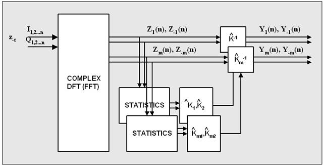
In the implementation of the process the expectation has been substituted by an average in time and in frequency using nearby frequency pairs.

Fig.6 –Block diagram of AIQB processing

The effect of AIQB algorithm on the signal of fig.4 is shown here:

Fig.7 – CIAOradio output with AIQB (test signal 1)

The test signal setup used during the AIQB implementation has been made by Claudio Re, I1RFQ.

The test1 signal used in Fig.4 and Fig.7 is a single generator sweeped by a low frequency FM modulation span of 22 kHz .

The test2 signal used in Fig.8 and Fig.8 is a single generator sweeped by a low frequency FM modulation span of 11 kHz.

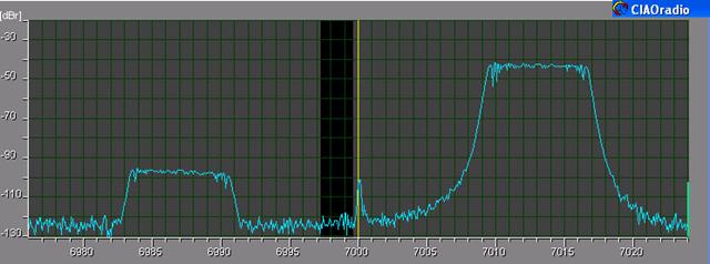
Fig.8 – CIAOradio output imbalance (test signal 2)

The imbalance without AIQB is around – 50 dB

Fig.9 – CIAOradio output imbalance with AIQB (test signal 2)

With the AIQB active the imbalance decreases up to -80 dB, with a 30 dB improvement.

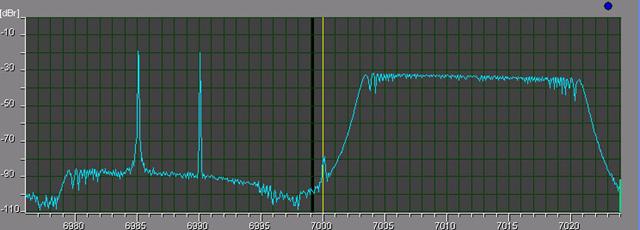
The test3 signal used in next measure is obtained summing the output of 3 RF generators.

One generates a 18kHz sweeped FM at 7012, while the other two generate sinewave at 6985 kHz and 6990 kHz, placed at opposite side of Fo.

Fig.10 – CIAOradio output imbalance (test signal 3)

Fig.11 – CIAOradio output imbalance with AIQB (test signal 3)

AIQB has been described. This algorithm has been implemented and adjusted in CIAOradio program. The version tested in this document is program version 1.42alfa.

The performance of the algorithm is interesting. It do not require any special test signal and the only requirement is that signal and its image are uncorrelated.

The high balance obtained could be used to implement direct low IF conversion receiver up to microwaves frequency range.

Further investigation on the performance optimization and in reducing computing power is planned.

References:

[1] http://www.comsoc.org/tech_focus/pdfs/rf2/pdf/23.pdf

Frequency Offset and I/Q Imbalance Compensation for Direct-Conversion Receivers

Guanbin Xing, Manyuan Shen, and Hui Liu, IEEE TRANSACTIONS ON WIRELESS COMMUNICATIONS, VOL. 4, NO. 2, MARCH 2005

[2] http://www.ifn.et.tu-dresden.de/MNS/veroeffentlichungen/2004/Windisch_M_INOWO_04.pdf

Standard-Independent I/Q Imbalance compensation in OFDM Direct-Conversion Receivers

Marcus Windisch, Gerhard Fettweis Dresden University of Technology, Vodafone Chair Mobile Communications Systems, D-01062 Dresden, Germany.

[3] http://wwwmns.ifn.et.tu-dresden.de//publications/2004/Windisch_M_ISCCSP_04a.pdf

BLIND I/Q IMBALANCE PARAMETER ESTIMATION AND COMPENSATION

IN LOW-IF RECEIVERS Marcus Windisch, Gerhard Fettweis Technische Universit¨at Dresden, Vodafone Chair Mobile Communications Systems, 01062 Dresden, Germany.

[4] http://wwwmns.ifn.et.tu-dresden.de//publications/2004/Windisch_M_ISCCSP_04b.pdf

PERFORMANCE ANALYSIS FOR BLIND I/Q IMBALANCE COMPENSATION

IN LOW-IF RECEIVERS Marcus Windisch, Gerhard Fettweis Technische Universit¨at Dresden, Vodafone Chair Mobile Communications Systems, 01062 Dresden, Germany.

[5] http://www.flex-radio.com/

The SDR-1000, from Flexradio. is a complete Software Defined Radio (SDR) transceiver interface to a Personal Computer. Gerald Youngblood, K5SDR

[6] http://www.proaxis.com/~boblark/dsp10.htm

The DSP-10 is an amateur-radio, software-defined 2-meter transceiver that can be built at home.

Bob Larkin, W7PUA

[7] http://www.sdradio.org/ or http://www.weaksignals.com/ -“Here you can find my software, developed for radio amateur's use, all freeware. “

Alberto Di Bene, I2PHD

[8] http://www.moetronix.com/spectravue.htm

A Windows based Spectral Analysis/Receiver Program. Moe Wheatley AE4JY

[9 ] http://www.sm5bsz.com/linuxdsp/linrad.htm - “ ... In case the input signal is in complex format Linrad has routines to correct amplitude and phase for complex input signals These routines operate in the frequency domain and can absorb frequency dependent phase and amplitude errors that are introduced by differences in amplifiers and filters used between the I/Q mixers and the audio board. The only requirement (non trivial) is that amplitude and phase errors are independent of amplitude, time and temperature.”

Leif Åsbrik, SM5BSZ

[10 ] http://www.dxatlas.com/rocky/

“…I/Q Balancing in Rocky is fully automatic and does not require any lab equipment, all you have to do is start the program when the band is open. Rocky will use all strong stations on the band as signal generators! The algorithm works as follows. The power spectrum is scanned for the signals that are at least 30 dB above the noise. For each signal, synchronous detection of the image is performed using the main signal as a reference oscillator. “

Alex VE3NEA, VE3NEA

[11] http://en.wikipedia.org/wiki/Expected_value

From Wikipedia: In probability theory the expected value (or mathematical expectation) of a random variable is the sum of the probability of each possible outcome of the experiment multiplied by its payoff ("value").

[12] http://www.comsistel.com/Ciao%20Radio.htm

CIAOradio SDR Oscar Steila IK1XPV , Claudio Re I1RFQ.

Homepage: www.qsl.net\ik1xpv

e-mail: [email protected]